Real-Time Analytics With Presto & Apache Pinot: Part 1

Read Real-time Analytics with Presto and Apache Pinot — Part II

In this world, most analytics products either focus on ad-hoc analytics, which requires query flexibility without guaranteed latency, or low latency analytics with limited query capability. In this blog, we will explore how to get the best of both worlds using Apache Pinot and Presto.

Today’s compromises: Latency vs. Flexibility

Let’s take a step back and see how we analyze data with different trade-offs.

Flexibility takes time

Let’s assume your raw data is hosted in a data lake available for users to process using Spark/Hadoop compute jobs or from the SQL engine.

In this case, users have full flexibility to access all of the data, pick whatever they want, and apply whatever computations they need.

However, it takes a long time to retrieve the results, as raw data is read from a data lake(s3/HDFS/etc.), and the computations are launched on-demand (in an ad-hoc manner).

Take this simple example on Presto: an e-commerce business has a dimension table of user information (100k rows with schema <customer_id, name, gender, country, state, city, …>) and a fact table of user orders(1 billion rows with schema <order_id, date, customer_id, items, amount>).

To find the monthly sales of all female customers in California, we need to write a SQL query to join the two tables and then aggregate the results.

This query execution has 4 phases:

1. The table scanning phase scans data from both tables: one full scan on table orders with columns: <date, customer_id, amount> And another full scan on table customers to fetch all the matched <customers_id, city> given predicate <state = ‘California’ AND gender = ‘Female’>.
2. The join phase shuffles the data from both tables based on customer_id.
3. The group-by phase again shuffles data based on <orders.date, customers.city>, then aggregate order amount.
4. Reduce phase collects all the group-by results and renders the final results.

The data shuffling phase contributes majorly to the query latency, including data partitioning, serialization, network i/o, deserialization.

ETL trades off data freshness for low query time

To optimize the query performance, ETL comes to the rescue. In ETL jobs, users can pre-join the fact table to the dimension table and then query it on the ETL’ed table.

Pre-joined table

In the above example, we can pre-join the users table and orders table to a new table user_orders_joined (which translates to 1Billion rows with schema: <order_id, date, customer_id, amount, gender, state, city>).

Then the above query can be written directly on this table:

In this case, we can compute metrics related to the order amount and do slicing and dicing on user dimensions like gender, location, and time. E.g., what’s the average amount of orders per month for male customers in Los Angeles.

The downside of a pre-joined table is that the query time is still proportional to the total number of rows scanned. In the above example, if there are 1 million rows that match the predicate of WHERE state = ‘California’ AND gender = ‘Female’ then, 1Million additions happen to compute the final results.

Pre-aggregated table

A noticeable improvement from the above approach is to pre-aggregate the results we want to query, e.g., we can create a new table user_orders_aggregated, with schema: <date, gender, state, city, sum_amount, sum_sold_items, avg_amount, …>. Assuming there are 1 million unique combinations of date/gender/location per month, the total number of records after pre-aggregation could be reduced to 12 Million rows for one year worth of data.

In this case, we pre-aggregated data based on user dimensions (gender, location, etc.) and order date. Then for each combination, we also compute all the corresponded metrics.

So we can rewrite the above query to:

In this query, the number of additions we do is just the number of dates in this table.

Pre-aggregation reduces a lot of runtime query workload compared to the previous approach. However, it still requires some runtime aggregations. The number of records scanned is proportional to the multiplication of cardinalities of non-group by columns in the table(after the predicate).

Pre-cubed table

Pre-cubing is the solution to achieve constant query latency. Users can pre-compute all the metrics we are interested in based on all the dimension combinations, so for any query, it will always be an exact row to answer it. For the above example, we can create a new table user_orders_cubed (1 Million rows with schema: <date, month, gender, state, city, sum_amount, avg_amount, …>)

So the above query can be rewritten to:

The downside of the pre-cubing solution is that the dataset size is the multiplication of all the dimensions cardinalities. If we add a new dimension with a cardinality of 10, then the number of rows will be ten times. This approach will not scale with organic growth of data size and the number of dimensions.

How to not trade-off using Apache Pinot

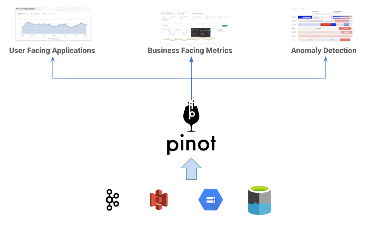
Apache Pinot is an OLAP data store built within LinkedIn for low latency analytics.

Here, low latency itself is referring to both low ingestion latency as well as low query latency.

For low ingestion latency, Pinot can directly consume from streaming data sources( Apache Kafka/Kinesis), and the events will be queryable immediately. Apart from Kafka, Pinot could batch load data natively with Pinot Minion Tasks from blob stores like HDFS, Amazon S3, Google Cloud Storage, and Azure DataLake Storage. There are also libraries around Hadoop and Spark jobs to use external compute resources for data bootstrap or routine ingestion.

Pinot has implemented multiple index technologies like sorted index, inverted index, bloom filter, star-tree index to speed up queries for low query latency.

Pinot has also been widely adopted by many companies like Uber, Weibo, Slack for user-facing applications, business analytics, and anomaly detection use cases.

In production environments, Pinot handles the workload of ingesting millions of events per second and serving thousands of queries per second with milliseconds level latency.

Apache Pinot proposed a creative solution to optimize scenario 3 in the above section by introducing Star-Tree indexing, which allows the user to configure maximum rows scanned for answering a query (beyond which results are pre-aggregated). Users can thus find a good balance between execution time and storage space requirements [ 1].

Resources

Next, we will discuss how to integrate Presto and Pinot to solve this problem in Real-time Analytics with Presto and Apache Pinot — Part II. Also, feel free to jump to Pinot Kubernetes Quickstart [ 2] for deploying Presto and Pinot in practice.

• Please visit the Apache Pinot Website and Documentations for more information and tutorials.
• Please join Apache Pinot Slack for news, questions, and discussions.
• Please join Apache Pinot Meetup Group for future events and tech talks!
• Follow us on Twitter: https://twitter.com/startreedata
• Subscribe to our YouTube channel: https://www.youtube.com/startreedata

Reference

[ 1] Star-tree index: Powering fast aggregations on Pinot

[ 2] Pinot Kubernetes Quickstart