Apache Pinot 101: Lesson 4 - Indexes for Faster Queries

This is the fourth lesson in the Apache Pinot 101 Tutorial Series:

• Lesson 1: Up and Running with Docker
• Lesson 2: Ingesting Data with Kafka
• Lesson 3: Ingesting Batch Data
• Lesson 4: Indexes for Faster Queries
• Lesson 5: Queries with SQL, Joins
• Lesson 6: Visualization with Superset

Indexes enable faster and more targeted data retrieval, significantly improving query performance. This lesson covers some of the index types that Pinot offers and then walks you through the process of creating your own index.

Pinot provides a variety of index types, each designed for specific use cases and data characteristics. The various types of indexes include:

• Bloomfilter index 
• Forward index 
• Geospatial index 
• Inverted index 
• JSON index 
• Range index 
• Startree index 
• Text index 
• Timestamp index

By understanding the properties and trade-offs of each index type, you can choose the most appropriate one for your particular data and query patterns. There are more details about how to use the different index types in the docs. For this lesson, you’ll use the range index to efficiently query over a range of price values.

The range index allows optimizing queries that filter over a range of values. A good example of this is the price column. To find out the number of times the price of Bitcoin went past 87000, we’d write the following query:

SELECT COUNT(*)
FROM ticker
WHERE price >= 87000;

In the absence of an index, the query would need to check all the rows that we’ve ingested. The range index will speed up queries that use comparison operators.

To create a range index, add the name of the column – in this case price – to rangeIndexColumns under tableIndexConfig.

{
    "tableIndexConfig": {
        "rangeIndexColumns": [
            "price"
        ],
        ...
    }
}

Once we’ve updated our table configuration, we’ll make a curl request to send it to Pinot. Then we’ll reload the segments so that the index is created.

Pinot provides flexibility when it comes to index creation. You have the option to create indexes either before or after you’ve ingested data into the system. This means that if you initially ingest data without creating specific indexes, you’re not locked out of optimizing your queries later.

If you decide to add indexes after data has already been ingested, Pinot doesn’t require you to re-ingest the entire dataset. Instead, you can simply refresh the segments. This refresh process allows Pinot to incorporate the new index structures into the existing data, making them available for use in subsequent queries. This flexibility in index creation and management simplifies the process of optimizing query performance without disrupting the data ingestion pipeline.

Execute the following curl command to PUT the updated table configuration.

curl -XPUT -H 'Content-Type: application/json' -d @tables/001-ticker/ticker_table.json localhost:9000/tables/ticker

Next, reload the segments of the table.

curl -XPOST localhost:9000/segments/ticker/reload

The index should now be used next time the query is run. This can be confirmed with explain plan:

EXPLAIN PLAN FOR
SELECT COUNT(*)
FROM ticker
WHERE price >= 87000;

In the output, the FILTER_RANGE_INDEX operator is now being used. This indicates that the range index was used to search for rows where the price was greater than or equal to 87000.

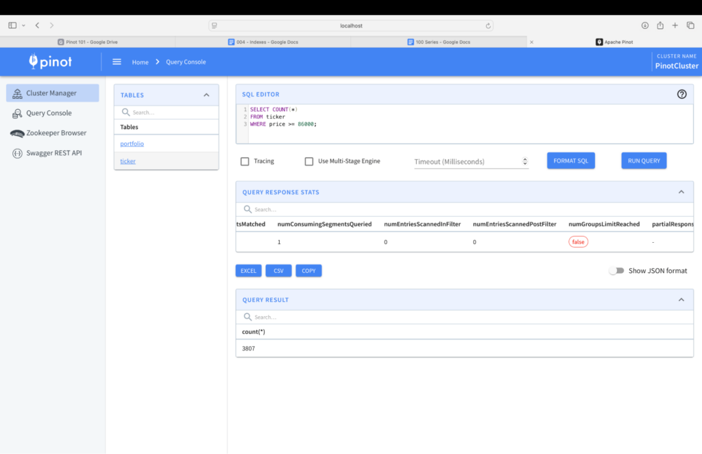
To confirm that the index did help in selectively picking the rows to scan, here’s some metrics with and without the index. Specifically, look at the numEntriesScannedInFilter metric when the query is run with and without index. Without index, this matches the total number of rows.

With index, however, the engine is very selective with the rows it retrieves. We see, in the image below, that numEntriesScannedInFilter is 0 which indicates that all predicates in the query had an index applied to them.

That’s it on how to create an index to speed up the queries. In this post we’ve seen how to use the range index. Pinot comes with various types of indexes that speed up different types of queries.

In the next lesson, you’ll see more on how to write queries and find the current value of a Bitcoin portfolio

Next Lesson: Queries with SQL, Joins →