What Makes Apache Pinot Fast: Chapter 2

Chapter II – The Power of Indexing

Introduction

In chapter 1 of this blog series, we recalibrated our understanding of “fast” in real-time analytics, as ultra-low latency in the order of milliseconds, even at extremely high throughput. We introduced Apache Pinot and brushed over-optimization techniques that give Pinot the ability to meet these new latencies and throughput requirements.

In this chapter, we will begin to explore filter and aggregation optimizations, by reviewing all the indexing techniques that are available in Pinot. We’ll look at some of the use cases where each index would be a great fit, and see some benchmarks demonstrating the astounding impact those indexes have on query latency.

The Power of Indexing

As we briefly saw in Chapter I, filter and aggregation optimizations reduce the amount of work needed to process a Pinot segment. As you may recall, a Pinot segment represents a subset of the input data along with column indexes. Indexes help in minimizing the data scans on corresponding columns during query processing and help retrieve the required values quickly. This helps in accelerating filter predicates, where we need to locate rows that match the specified predicate. This also helps in speeding up aggregation functions, where pre-aggregation can help avoid on-the-fly processing overhead. Adding an appropriate index based on the use case provides orders of magnitude performance improvements in query latency as well as overall throughput.

Indexes in Pinot

Pinot has a rich set of indexes. They range from the familiar general-purpose ones such as inverted index, sorted index and range index, all the way to specialized ones such as Startree index and JSON index. Each index has its own advantages, depending on the query patterns and use case. For any given column in a Pinot table, we can apply any of these indexes. The query processing layer is then able to generate a per-segment query plan to leverage such indexes for segment-level processing , which in turn accelerates the overall query performance.

Let’s go through the list of indexes available in Pinot today. For each index, we talk about the inner workings and the benchmarking numbers comparing query performance with and without that particular index.

Inverted Index

As the name implies, an inverted index maintains a map of each column value to its location using an efficient bitmap. For columns that are frequently used in the filter predicates, configuring an inverted index can directly identify the location of the value specified in the query. This helps in drastically reducing the number of scans required and hence improves query performance. More details about how this works can be found in the Inverted Index section of the Pinot documentation.

Below is a comparison of query latency, for an aggregation query with a filter predicate, on a dataset with ~3 billion rows. Without inverted indexing, the query had to do a full scan of 3 billion rows and took over 2.3s , whereas after applying an inverted index the latency dropped to just 12ms!

Fig: Aggregation query with filter on ~3 billion rows dataset. Count the number of events for a given actor_id

Inverted indexes are very effective for arbitrary slice and dice, because of which use cases like user-facing analytics, metrics, root cause analysis, and dashboarding greatly benefit from them.

Sorted Index

One column within a Pinot table can be configured to have a sorted index. Internally, it uses run-length encoding to capture the start and end location pointers for a given column value, thus drastically reducing scans and in turn decreasing query processing time. For more details, refer to the Sorted Index section in the Pinot documentation.

Below is a comparison of query latency, for an aggregation query with a filter predicate, on a dataset with ~3 billion rows. Without indexing, the query had to do a full scan of 3 billion rows and took over 2.3s, whereas after creating a sorted index the latency dropped to just 15ms!

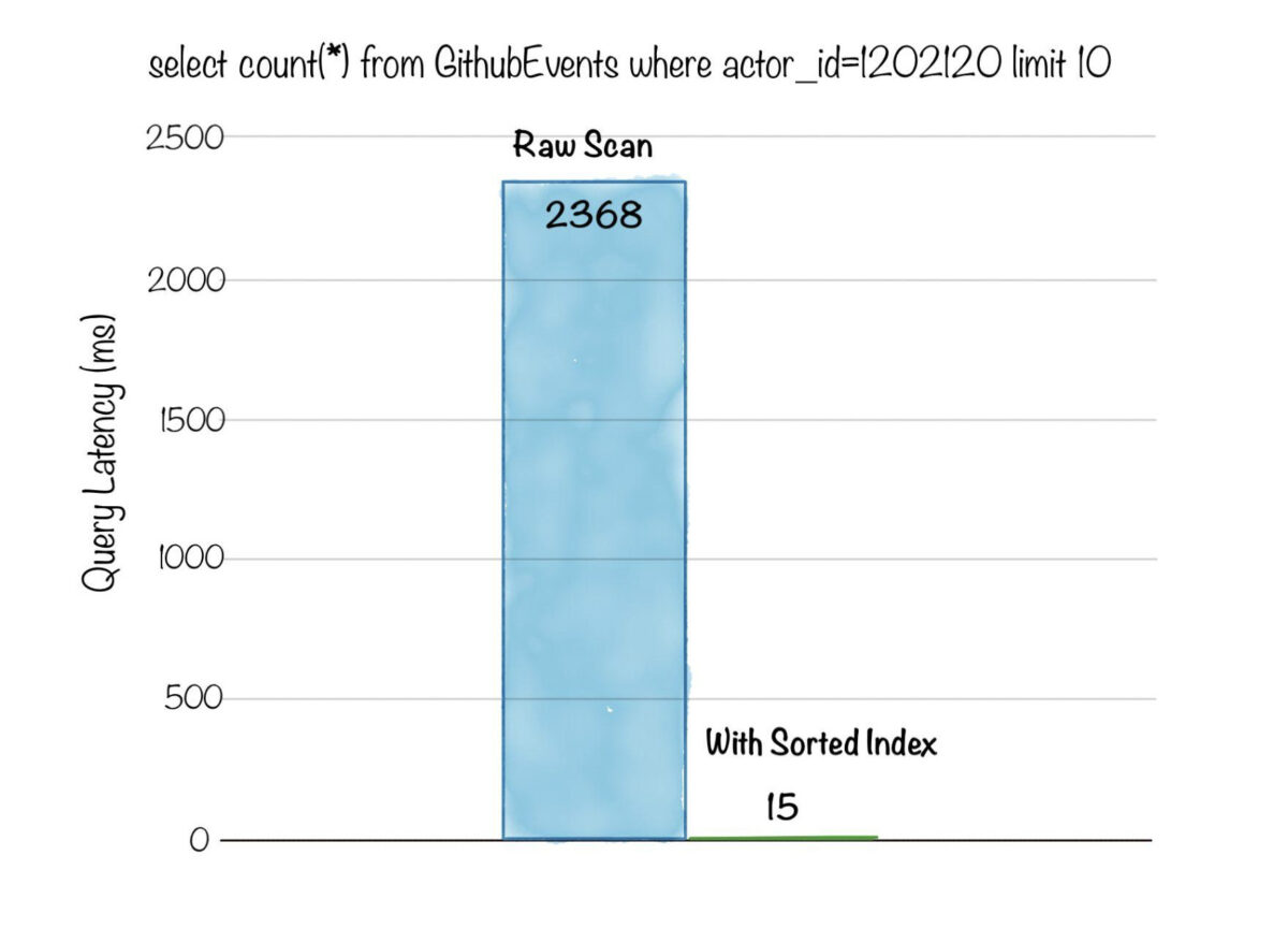
Fig: Aggregation query with filter on ~3 billion rows dataset. Count the number of events for a given actor_id

Sorted indexes are most effective for use cases like personalization and user-facing analytics. Datasets in such use cases tend to have a primary entity (such as a memberId, companyId, jobId) that the majority of the queries include in their filter predicates.

Range Index

Range index is a variant of inverted index that can speed up range queries i.e. queries with range predicates (e.g. column > value1, column <= value2). In the case of columns that contain a large number of unique values, the range index leads to faster query performance and more efficient representation for such range queries. Head over to the Range Index section in the documentation for more details.

Below is a comparison of query latency, for an aggregation query with a range filter predicate on a numeric column, on a dataset with ~3 billion rows. Without range indexing, the query had to do a full scan of 3 billion rows and took over 40s , whereas after range indexing was applied, the latency was reduced to just 2.9s!

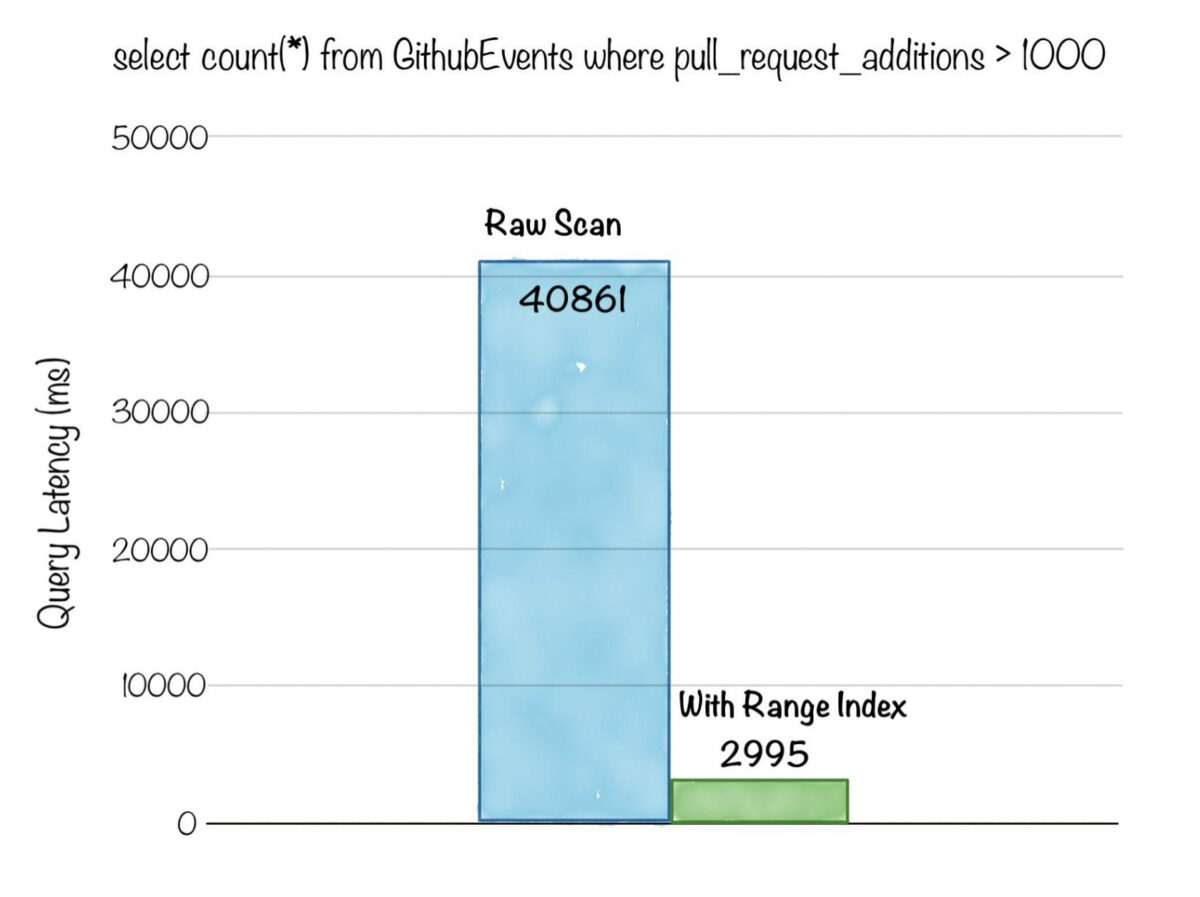
Fig: Aggregation query with range filter on ~3 billion rows dataset. Count the number of events where additions per pull request is > 1000

Range indexes are extremely useful in speeding up queries for use cases such as anomaly detection, root cause analysis, and visualization dashboards. These use cases tend to have time-series data, or data with several metric columns, and often need fast slicing and dicing for specific numeric ranges.

JSON Index

Pinot enables storing a JSON payload representing arbitrarily nested data as a String column, which is then available for query processing. A JSON index can be applied to such columns to accelerate the value lookup and filtering for the column. This is a very powerful feature that lets you index all fields within your nested JSON blob, and thus remove the need for ingestion-time or query-time transformations. Details on how this works can be found in the JSON index section.

Below is a comparison of query latency, for a selection query with a filter applied on a field inside the nested JSON column. Without JSON indexing, the query had to do a full scan of 100M rows and parse the JSON string in each row, taking over 17s. After applying the JSON index, the query took only 10ms!

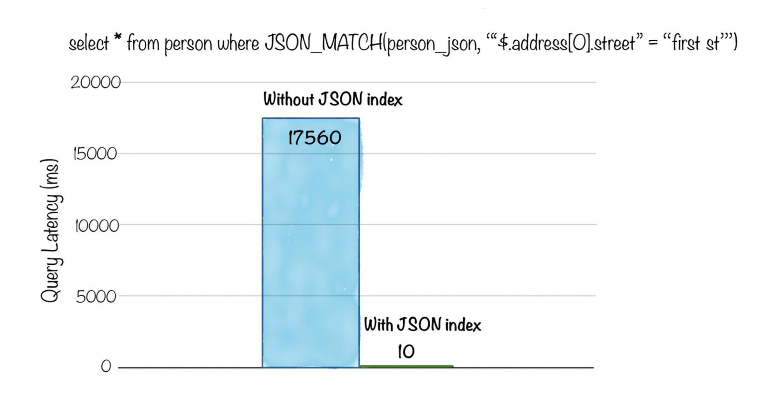
Fig: Selection query with JSON match on ~100M rows dataset. Select the rows for persons who live on “first st”

Text Index

Pinot provides the ability to do a regex-based text search or fuzzy text search on String columns using a text index. Internally, this is implemented using an Apache Lucene index. This enables fast query processing on unstructured text columns, for a variety of text search categories, such as term or phrase search, prefix query search, regular expression query, and so on. To read more about this index, head over to the Text Index section in the documentation.

Below is a comparison of query latency, for a selection query with text match, on a dataset with ~3 billion rows. Without a text index, the query had to scan all rows and apply a UDF for identifying the text match and took over 15s . After applying the text index, the query took only 126ms!

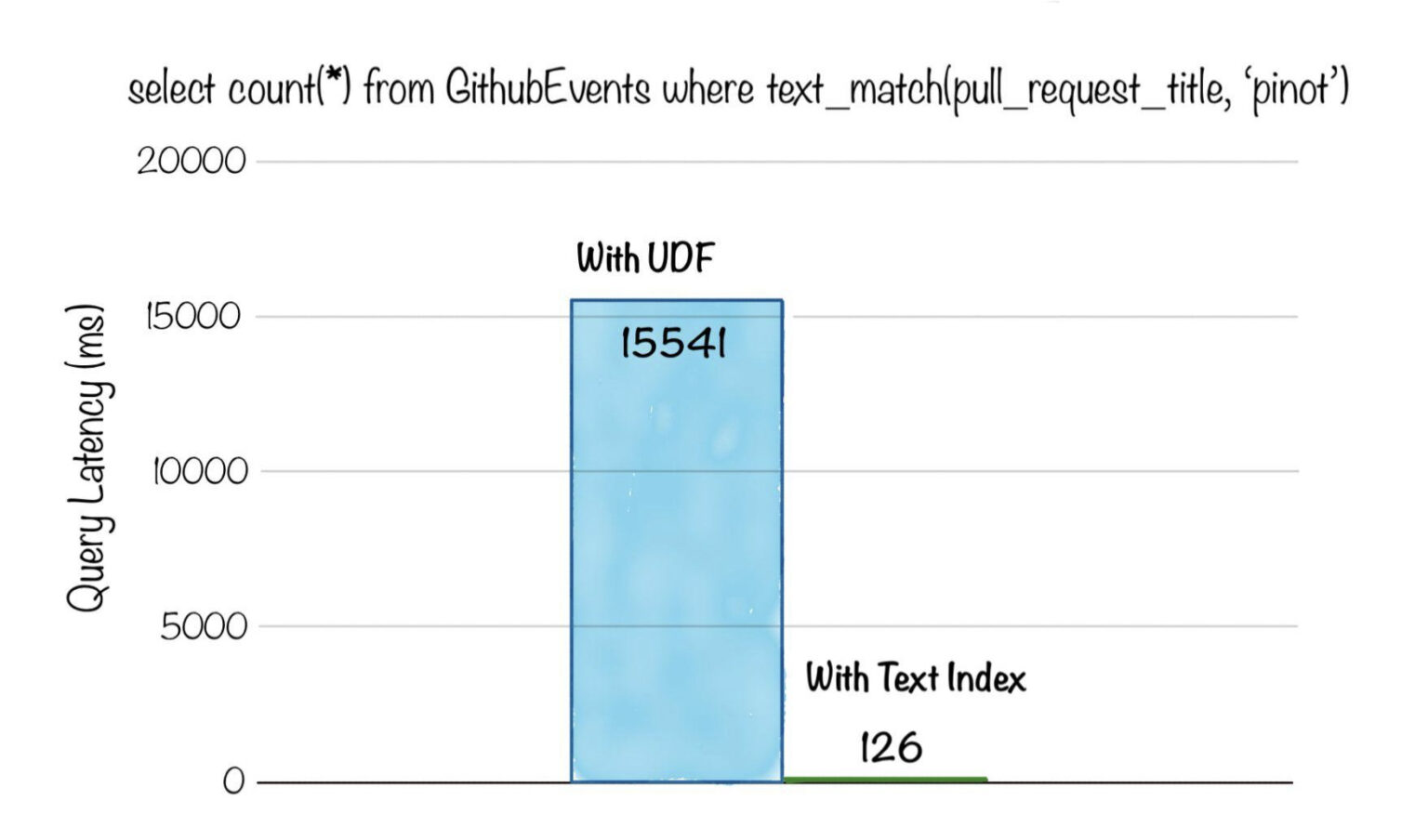
Fig: Aggregation query with text search filter on ~3 billion rows dataset. Count the number of events for pull requests with ‘pinot’ in the title

As we can see from the two benchmarks above, JSON index and text index allow querying unstructured data without the need for expensive UDFs and application side results post-processing. This is especially useful in use cases like user-facing analytics, personalization, log analytics, text search, and ad hoc analytics , where there’s little control on the structure of the data generated.

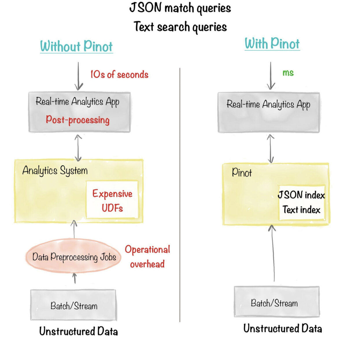
Fig: JSON index, text index eliminates the need for expensive UDFs and application side results post-processing

GeoSpatial Index

Many use cases often need the ability to do geo-spatial queries, such as filter records that fall in a given geo-fence (i.e. in a specified area on a map) based on their corresponding latitude and longitude values. Pinot’s Geo-Spatial index is used to accelerate such queries. Internally, it is implemented using Uber’s H3 library and supports a variety of geospatial data types and functions natively. More details can be found in the Geospatial Index section.

Below is a comparison of query latency, for a selection query with a filter to find rows having a geo-location within a radius of a specific point. Without the geospatial index, the query had to scan all rows and apply a UDF to compute the distance, taking 1s to execute. After applying the geospatial index, the query latency dropped to just 50ms!

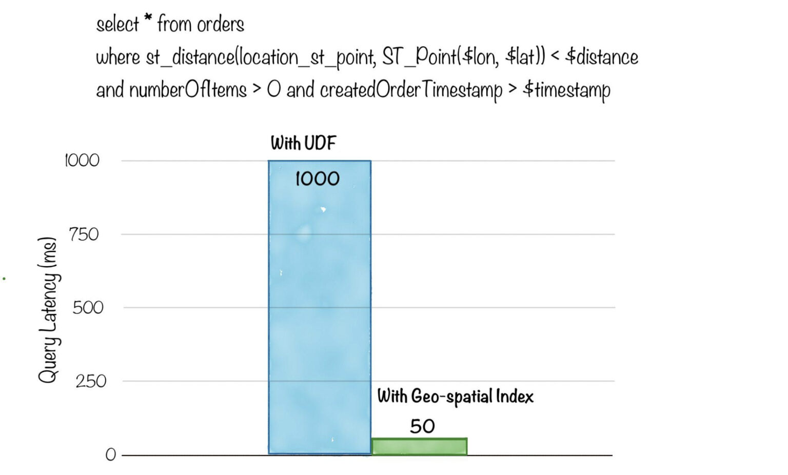
Fig: Geo-spatial queries on 1 billion rows to find events happening nearby a given geo-location. Reference ‘Orders Near You’ and User-Facing Analytics on Real-Time Geospatial Data

The geospatial index is very useful to ensure that applications can render complex geospatial visualizations , such as scatter plots & world maps, with low latency and without additional application side data pre-processing or post-processing overhead.

StarTree Index

StarTree is a special type of index that serves as a filter as well as an aggregation optimization technique. StarTree takes in a list of dimensions and aggregation functions. For each unique dimension combination, StarTree pre-computes and stores the aggregate metric values. Startree lets you specify exactly which dimensions to pre-compute and how many values to pre-compute – effectively providing a tunable knob between storage space and query latency. For high cardinality columns, we can bound the number of scans needed to satisfy the corresponding query using this knob and therefore, achieve predictable query latency. You can find more details in our documentation in the StarTree Index section.

Below is a comparison of query latency, for an aggregation query with a filter predicate, on a dataset with ~3 billion rows. Without indexing, the query had to do a full scan of 3 billion rows and took over 31s , whereas after generating the StarTree index the latency reduced to just 50ms!

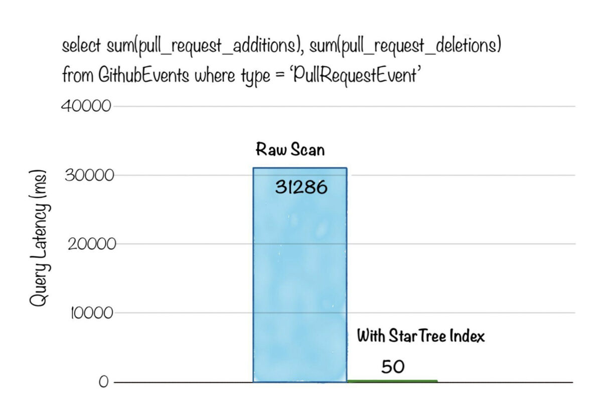
Fig: Aggregation query with filter on ~3 billion rows dataset. Get SUM of additions and deletions to pull request for a given type of event

StarTree index is an excellent choice for use cases such as anomaly detection, root cause analysis, user-facing analytics, that need fast aggregations with point lookups on arbitrary dimension combinations.

As shown in the diagram below, OLAP systems that don’t have the StarTree index have to resort to pre-processing the input data, to compute aggregate values for a combinatorial explosion of keys. Needless to say, this adds tremendous overhead on use case onboarding as well as day to day maintenance to keep these aggregate values consistent with the data source

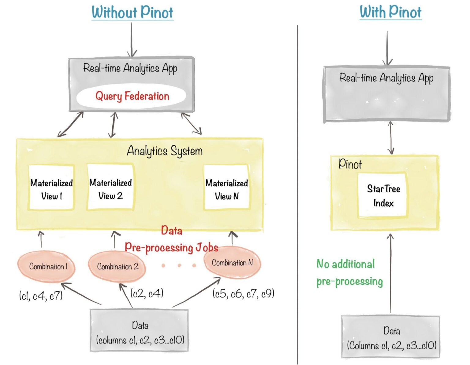
Fig: Without StarTree index, one complex data pre-processing job is needed per materialized view, and the responsibility of federating queries across the views falls on the application.

Enabling Indexes

It is very easy to enable and get started with indexing in Pinot. Indexing is enabled by simply specifying the desired column names in the table config. More details about how to configure each type of index can be found in the Indexing section of the documentation.

There are 2 ways to create indexes for a Pinot table. They can be created as part of the ingestion, during Pinot segment generation. Alternatively, they can also be dynamically added to segments or removed from segments at any point, by updating the config and invoking a reload segments API. Instructions for this can be found in the Enabling Indexes section from the documentation.

Stay Tuned

We hope you enjoyed reading this overview about all the indexes available in Pinot. Pinot’s indexes play a major part in making Pinot blazing-fast, thus allowing it to support a wide spectrum of real-time analytics use cases and push the boundaries of latency, throughput, and scale. We will release deep-dive blogs for many of these indexes to discuss interesting design considerations, implementation-specific details, and real-world use-cases that they solved. We will also publish more chapters in this series, each putting a spotlight on other optimization techniques in Pinot. Stay tuned!

We’d love to hear from you

Here are some ways to get in touch with us!

Ping us on Slack with your questions, comments, and ideas. Here’s a great resource to help you get started with Apache Pinot . Engage with us on Twitter, we’re at StarTree or ApachePinot. For more such content, check out our Blogs page, subscribe to our Youtube Channel, or catch us at an upcoming meetup.