
The definition of real-time analytics has evolved drastically in the recent few years. Analytics is no longer just ad-hoc queries and dashboards, with lenient SLAs, for a handful of internal users. Companies now want to support complex real-time analytics use cases, such as user-facing analytics, personalization, anomaly detection, root cause analysis. This has dramatically changed the expectations of query latency, throughput, query accuracy, data freshness, and query flexibility from underlying analytics systems. This blog How to Pick Your Real-time OLAP Platform – Part I does an excellent job of describing all these new use cases, the challenges they bring, and aptly quantifies the redefined expectations from underlying systems.
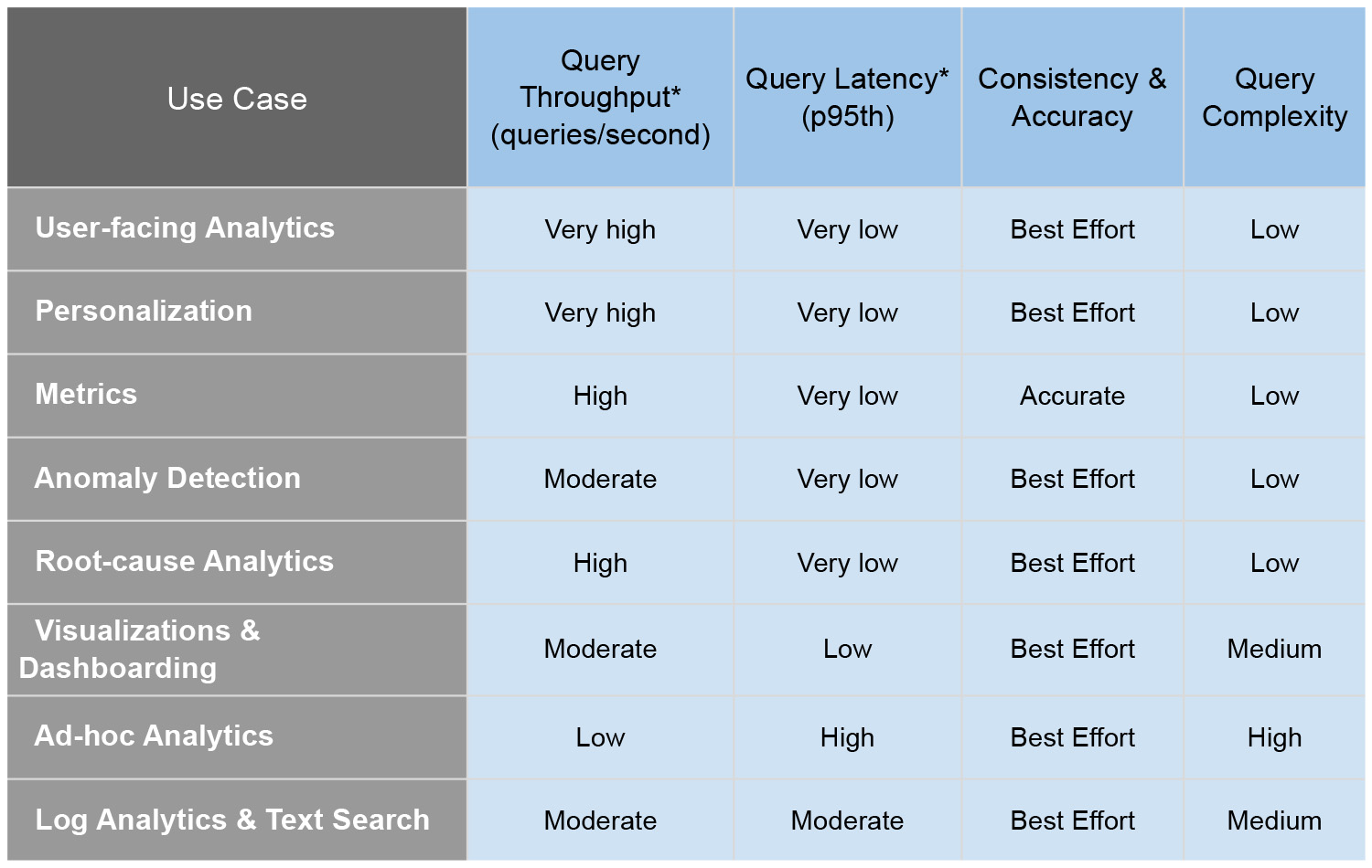
Image: Use case and associated query throughput, latency, consistency and accuracy, and complexity in a chart
*Query Throughput ranges: Very High = 10 – 100K; High = 100s – 10k; Moderate = 100s – 1k, Low = 10s – 100
*Query Latency Ranges: Very Low = 10 – 100ms, Low = 100ms, Moderate = Sub-seconds, High = 1 – 10s
Redefining fast
As we can see from the query latency column, in the real-time analytics land, “fast” now means ultra-low latency in the order of milliseconds, even at extremely high throughput. As customer bases start shifting from analysts & data scientists to end-users who are interacting directly with data products, the ability to respond with ultra-low latency even at extremely high query throughput becomes very crucial for the underlying analytics system.
Imagine you built an online food delivery app, and provided a dashboard to all restaurant owners, so that they can react in real-time to menu and demand fluctuations. Or that you built a social feed for millions of busy professionals and want to show them the most relevant and fresh content based on their real-time interactions. Or maybe, you built a dashboard to help dev-ops engineers investigate anomalous behaviors in key business metrics in real-time. Now imagine that for every interaction from your end-users your app spends several seconds being un-interactive because the many concurrent analytical queries triggered in the backend can only be served with seconds latencies by your analytical database. Such experiences directly result in low user engagement and poor session time, negatively impacting the company brand value and revenues.
So what’s the solution? How do we build interactive real-time analytical applications for modern-day end users?
Apache Pinot is really fast
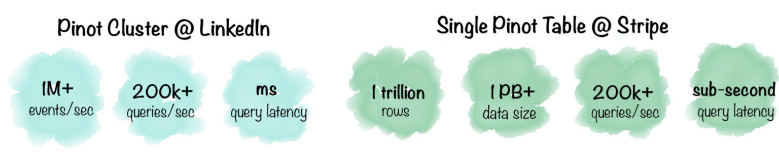
Apache Pinot is the perfect system to help you solve this problem. Apache Pinot is a distributed analytics datastore that was purpose-built for ultra-low latency high throughput real-time analytics. Originally developed in 2014 by engineers at LinkedIn and Uber for solving mission-critical real-time analytics use-cases, Pinot is now a very mature product today used by several companies for many different types of real-time analytics use-cases. Pinot powers LinkedIn’s feed impressions, Who Viewed My Profile, article analytics, Talent Insights, and many such use cases that require latency SLAs in milliseconds. The Pinot cluster at LinkedIn can handle upwards of 200k QPS while maintaining 100ms latency (p95th). Recently, Stripe spoke about their Pinot deployment which boasts of 200k+ QPS for a single table of 1PB+ data while maintaining sub-second latency. Pinot also powers several user-facing analytical applications in Uber, such as UberEats Restaurant Manager with 100s of QPS and <100ms (p99th) latency.
How does Pinot do this? What is the secret behind Pinot’s lightning-fast queries?
What makes Pinot fast?
At the heart of the system, Pinot is a columnar store with several smart optimizations that can be applied at various stages of the query by the different Pinot components. Some of the most commonly used and impactful optimizations are data partitioning strategies, segment assignment strategies, smart query routing techniques, a rich set of indexes for filter optimizations, and aggregation optimization techniques. Each of these techniques would make a highly interesting and detailed discussion on its own. We will be following up this blog post with a series of blogs, each going in-depth into one of these optimization techniques.
As for the rest of this blog, we’ll be doing a quick architecture recap and an overview of the query lifecycle, to set the context for the blogs that follow.
Quick Architecture Recap
If you’re already familiar with Pinot’s architecture, you can skip right ahead to the Query Lifecycle section.
Let’s take a look at the portions of Pinot’s architecture that are relevant for this blog series, mainly the Pinot table, segment, servers, and brokers.
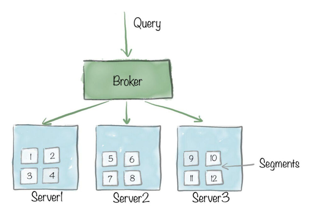
- Pinot table – a logical abstraction that represents a collection of related data, that is composed of columns and rows (known as documents in Pinot).
- Pinot segments – Similar to a shard/partition, data for a Pinot table is broken into multiple small chunks, that pack data in a columnar fashion along with dictionaries and indexes for the columns.
- Pinot servers – A node that is responsible for a set of Pinot segments, by storing them locally and processing them at query time.
- Pinot brokers – A node that receives user queries, scatters them to Pinot servers, and finally, merges and sends back the results gathered from Pinot servers.
Let’s double click into point 4 and see how the query travels from the user, through the different Pinot layers, and steps taken by Pinot at each layer to accelerate the query.
Query Lifecycle
The query begins at the broker, which retrieves the total set of Pinot segments and the Pinot servers containing those segments.
If no optimizations are applied, query processing will need to go through each segment on every server in the cluster and do scanning, filtering and aggregations. Pinot enables optimizations at various levels to reduce the amount of work needed per segment, as well as the total number of segments that need to be processed.
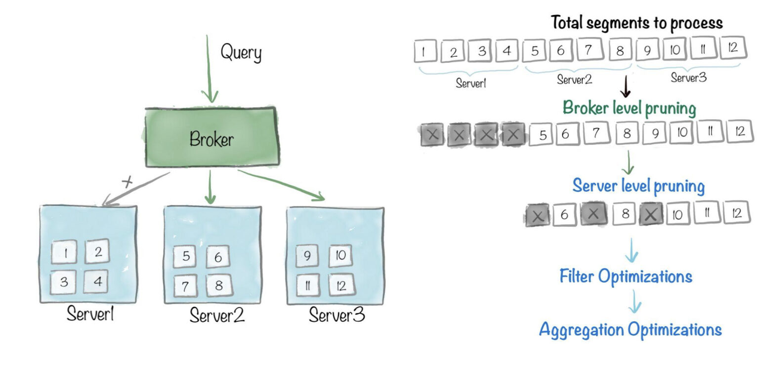
- Broker level pruning: At this stage, broker level pruning techniques – such as data partitioning, replica group segment assignment, partition-aware query routing – can be applied, to reduce this set of segments, and possibly the set of corresponding servers.
- Server level pruning: The query then makes its way to the servers, where server-level pruning techniques – such as metadata-based pruning or bloom filters – can be applied to further reduce the set of segments.
- Filter optimizations: Within each segment, indexing techniques can be applied on columns that have filter predicates, to reduce the total number of rows that need to be scanned within the segment.
- Aggregation optimizations: Finally aggregation optimizations can be applied, reducing the number of rows that need to be scanned to compute the aggregations present in the query.
Up Next
In the next chapter, we’ll be doing a deep dive into the indexing techniques available in Pinot. We’ll look at some of the use-cases where you would use them, and see some benchmarks demonstrating the astounding impact those indexes have on query latency. Stay tuned!
We’d love to hear from you
Here are some ways to get in touch with us!
Ping us on Slack with your questions, comments, and ideas. Here’s a great resource to help you get started with Apache Pinot. Engage with us on Twitter, we’re at StarTree or ApachePinot. For more such content, check out our Blogs page, subscribe to our Youtube Channel, or catch us at an upcoming meetup.