
How does one achieve OLAP functionality at the OLTP scale?
In other words, how do you open up a data warehouse to a user base of millions and let them query it to their heart’s content while maintaining millisecond-range latencies?
Even though it sounds very promising, delivering OLAP analytics at OLTP scale faces many challenges in practice. Latency is a significant problem as more concurrent users are introduced to the system. Getting those latencies back to tolerable levels requires an investment in additional infrastructure that is simply unsustainable. For example, we described how LinkedIn added hundreds of nodes to maintain latencies at a tolerable level.
While applications that deliver real-time user-facing analytics have brought this problem to the fore, it’s not the first time an organization has needed a solution that provided OLAP functionality at the OLTP scale.
This article explores several approaches to get faster OLAP analytics at scale, the challenges they bring in, and why Pinot was ultimately developed to overcome them.
A case in point
Before we dive deeper, let’s pick a specific case to set the stage for our discussion. This case was presented at Carnegie Mellon’s Vaccination Database talks for those interested.
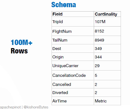
Suppose we have a data set from a major airline that includes flight arrival and departure details for commercial flights in the U.S. over two decades. That data has 100M+ rows, with fields such as a unique trip identification number (TripID), the flight number (FlightNum), origin and destination codes, etc.
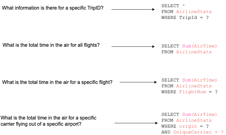
And here are examples of some of the queries one might run on this data:
Before Pinot: Raw Data, Pre-Join, Pre-Aggregate, and Pre-Cube
To answer the above questions, let’s consider four different approaches that could be used in a traditional OLAP database context.
- Raw data – Queries are run directly against the raw data.
- Pre-Join – Tables required to answer the query are joined beforehand.
- Pre-Aggregation – Columns included in the query are pre-aggregated.
- Pre-Cube – Each possible combination of the query result is pre-computed and materialized.
Let’s explore each approach in detail.
Querying raw data
Access to raw data gives a user (developer or an application) a tremendous amount of flexibility.
A person can potentially craft any query and apply it to the raw data when dealing with analytics. That will be a slow and inefficient process, as all the data must be sifted through at query time, making it difficult to achieve any scale, as throughput and latency suffer.
For example, in the airline example above each trip would be stored as a single row in the Trips table.
Pre-Joining tables
In scenarios where the query requires raw data to be processed across multiple tables, joins are required.
Doing join operations during query time adds to the overall query response latency. Pre-join reduces the response time in queries by joining the tables beforehand. However, this improvement can be achieved by knowing what data is likely to be required for a query and performing pre-join on the relevant tables.
For example, assume that we have a Flights table in the airline example to keep track of the information related to the aircraft used for the trip. It can contain dimensions like the flight number, model, seating capacity, etc., while the FlightNum serves as the primary key.
To find out all the trips made using a Boeing aircraft, we can join the Trips table with the Flights table using the FlightNum field. Typically, the join is performed using an ETL process and the result is written into a new table.
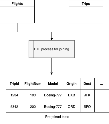
The next time a query is received, the result is directly served from the already joined table.
Pre-Aggregation
Here is one way to work with raw data every time: Simply pre-aggregate the data.
Another approach is to pre-aggregate the required fields based on the query.
The basic idea is to anticipate which analytics reports are most likely to be requested, then create a new table where the appropriate data has already been grouped (aggregated). Similar to pre-join, while there is still some runtime needed, pre-aggregation is an improvement over working with raw data if you know what queries and aggregations are likely to be submitted ahead of time.
For example, let’s consider the Trips and Flights tables in the airline example above.

The Flights table is a dimension table with a smaller number of records, whereas the Trips table is a fact table with 100M+ records.
Now let’s try to answer the following question:
What is the total time in the air for Boeing 777 flights?
Since the target metric, sum(Trips.AirTime), is known, the pre-join and pre-aggregation approach utilize an ETL process to join two tables and produce a pre-aggregated table called trips_flights_aggregated . We can remove unnecessary fields like tripId during pre-aggregation.
The trips_flights_aggregated table would look like the following.

The next time the query is received, it will be served faster as the data has already been aggregated.
Pre-Cubing
Yet, the fourth solution is called pre-cube, which is a special kind of pre-aggregation that matches what a user might want to query.
Pre-cube is, very loosely, a way of nesting aggregations. Assuming that there are only a few hundred unique combinations of various kinds of data, pre-cube can cut down the number of lines of data that need to be examined for a query by several orders of magnitude.
As far as our airline example is concerned, we can pre-compute each combination of dimensions upfront to save a lot of time at query execution. For example, the answers to the following questions can be pre-calculated and stored in a separate table or even in a key-value database like Cassandra or HBase.
- How many flights started from Atlanta?
- How many flights were made between Atlanta and San Francisco?
Benchmarking queries against each approach
Now let’s try to answer the questions asked in the airline example with each of these approaches described above.
Using a database and following the raw data approach, each trip would be stored as a single row. By contrast, a pre-aggregate approach would aggregate data across multiple trips based on some key attribute (dimension) and possibly remove columns that are not of interest. Finally, a pre-cube approach would pre-compute each possible cell (for example, the sum of AirTime for each flight number, destination, etc.).
The following is a comparison across query latencies against each approach…All these numbers were derived using Pinot.
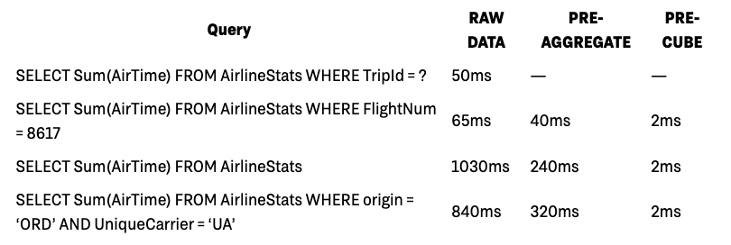
As you can see, the more complicated queries slow down considerably when working with raw data, whereas pre-cube stays relatively fast. Pre-aggregation is a compromise between the two.
Picking the right approach
As we witnessed above in the latency comparison, pre-cube seems like the hands-down winner for OLAP when complex queries are involved.
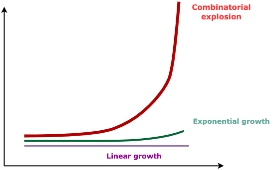
The issue, however, is that the pre-cube more than doubles the number of records that need to be stored (from 107M, it adds another 185M records). And so, while throughput is good, there will be a combinatorial explosion in the size of the database as the data volume and the cardinality of dimensions increase over time. That quickly becomes untenable in terms of investment.
[T]he Curse of Dimensionality]( https://en.wikipedia.org/wiki/Curse_of_dimensionality)
Moreover, when scaling analytics for user-facing applications, pre-aggregate and pre-cube run into a limitation: There is no knowing ahead of time what bits of information a user will be interested in, at what granularity, over what time frame. But the more potential queries the system needs to anticipate, the greater the storage needed for the data (among other things).
Choosing between the latency, flexibility, and throughput
All these limitations leave us no choice but to choose between latency, flexibility, and throughput. Different solutions often achieved one or two of these at the expense of the other(s).
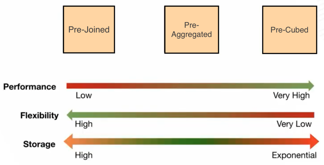
Whatever gains to be had in terms of latency and throughput (speed, if you will) are had at the cost of the flexibility of the system. And when there is less flexibility, there is tremendous pressure put on the hardware resources, making scaling unfeasible.
Different systems to address different use cases
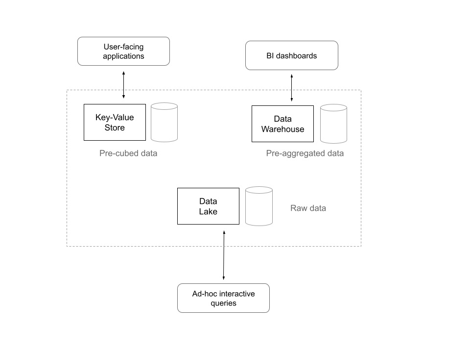
The variations in the space and time of data analytics have led the organizations to keep different systems to achieve different use cases.
For example, the results of the frequently accessed, predictable queries can be pre-cubed and stored in a key-value store. Later, they can be accessed by user-facing applications that demand low-latency reads. Also, data warehouses can keep pre-aggregated data sets and materialized views to be used for internal BI purposes. For those who want to work with raw data, a solution would be to use a data lake with an analytics engine like Hadoop, Spark, or Presto.
Although these different systems serve their intended purpose, they bring in many problems in practice. First, there’s data duplication across multiple systems. Moving data among systems takes substantial time and effort. Also, not to mention the management overhead added by them.
What if there’s one system that provides flexibility and speed with a single data set abstraction and is cost-effective?
That was the primary challenge that has led to the development of Pinot.
What Pinot brings to the table
Until the last few years, there did not need to be a solution to this problem. But necessity is the mother of invention: The rise of user-facing analytics, as well as the need for near-real-time data in OLAP systems, forced companies to invest in finding a solution.
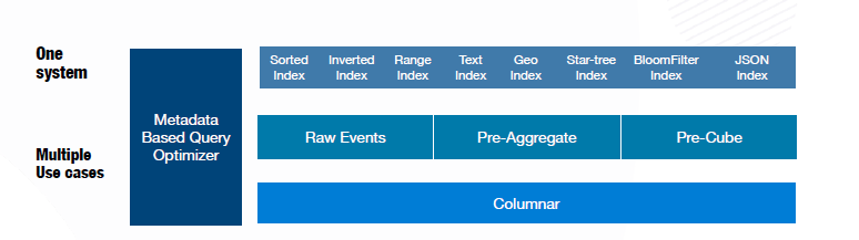
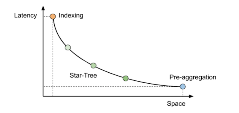
That is what gave rise to Pinot. Pinot can essentially triangulate between these approaches, automatically deciding which one will yield the best trade-off. The Pinot query engine optimizes those analytical query patterns (for example, filter/aggregations/group-by) using several different approaches. Additionally, Pinot can balance the storage of pre-cube data for specific queries by using special indexing techniques (star-tree index) for specific queries. In contrast, raw data can be made available for other queries.
For example, an organization could initially use Pinot to work with the raw data. When more data comes in and query throughput increases, additional indexes can be configured on raw data to speed up the queries. Additionally, Star Tree indexes can be enabled to gain more stringent query SLAs on the raw data set.
The bottom line is that Pinot allows you to walk from one end of the spectrum to the other end while still using the single data set. Unlike the approaches we discussed earlier, there’s no need to move data among systems to get analytics use cases done.
At the end of the day, Pinot is a single system that enables you to work on a single data set while giving you many control knobs to move between query flexibility in the raw data set fast and economical manner.
Pinot provides a single system with a single data set abstraction to address different use cases

For a more technical dive into how Pinot does this, we recommend the following sources: