Introduction

Query-time JOINs are a new capability in Apache Pinot, made possible by the Multi-Stage Query Engine. With Apache Pinot 1.0 we are thrilled to announce they are functionally complete, and now offer users a wider range of possible ways to gain insights from their data. In this article we will delve into the world of JOINs, discuss various optimizations we added in Apache Pinot for running fast and efficient JOINs, and highlight the best use cases for query-time JOINs.

Spectrum of data joins

Typically, organizational data is modeled using the star schema format. To obtain the highest quality and most performant insights from this data, executing joins on these tables becomes imperative. There are various approaches you can take when building applications that require such joined data. Each option comes with its own considerations of throughput, latency and flexibility, which affects the effectiveness of that approach for different types of analytics use cases. 

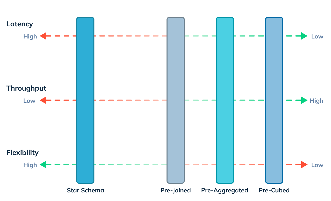
Figure 1: The various approaches when joining data – pre-cubing, pre-aggregating, pre-joining and star schema – and their implications on latency, throughput and flexibility.

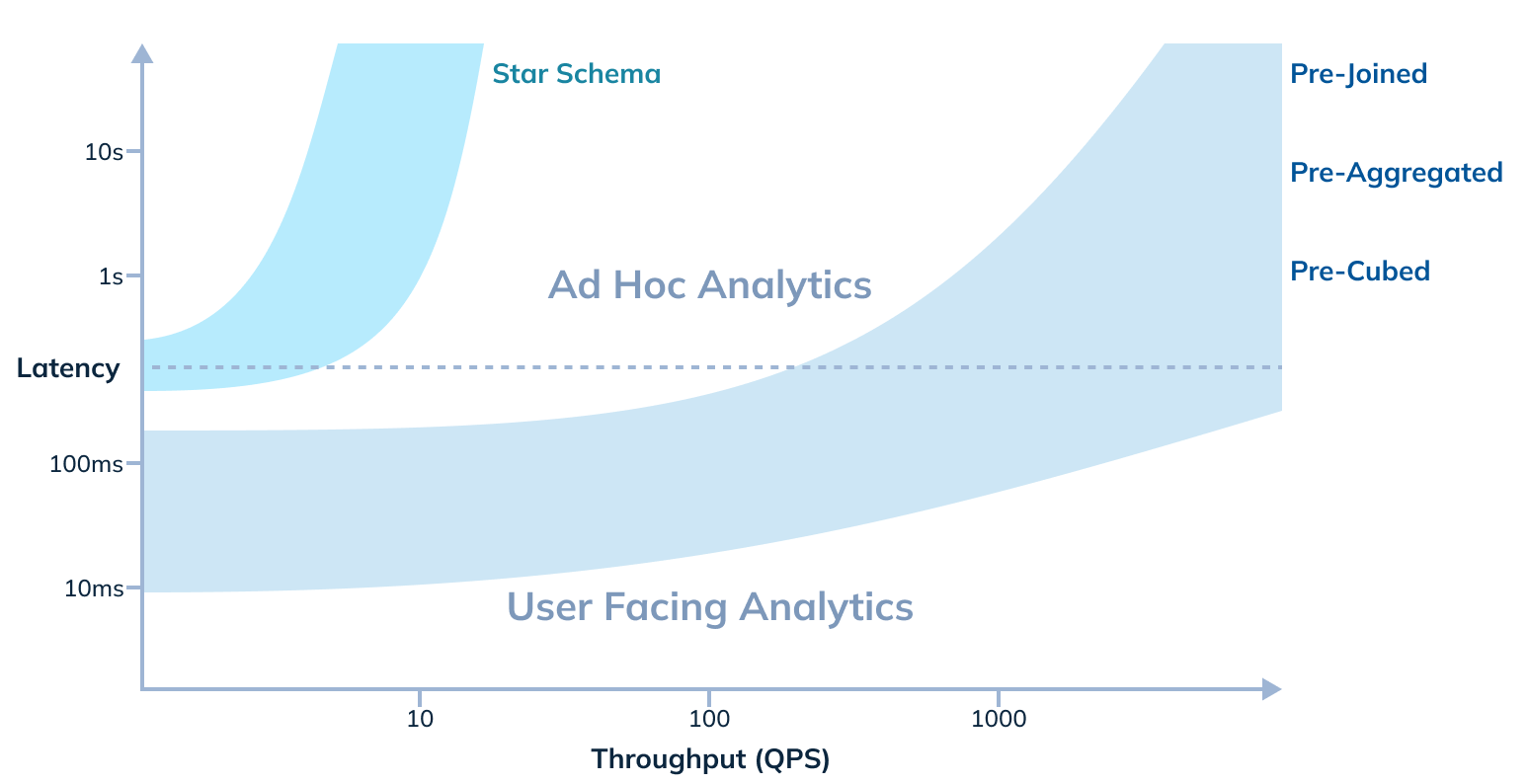
Figure 2: Ad hoc analytics – which is typically for internal users – is more accepting of higher latencies. On the other hand, user-facing analytics applications need to provide interactive and real-time experiences at end-user scale, thus requiring ultra-low latencies and very high throughput. The kind of analytics use cases that the system needs to support, will influence the choice of data modeling. 

Let’s walk through each of the approaches and evaluate their usability across ad hoc / user-facing analytics, based on where they fit in the latency vs. throughput graph. For the first three approaches, all / most of the data joining is happening at ingestion-time. For the last approach, the join is expected to be done at query-time.

• Pre-cube: Pre-cubing involves computing a data cube with all dimension combinations at any possible granularity, and to keep doing so incrementally. This results in high operational complexity and storage overhead. However, given all combinations are pre-computed, no data needs to be joined during query-time, thus achieving great throughput and latency. As shown in figure 2 above, this kind of data modeling can sometimes be done for user-facing analytics applications, where the datasets and query patterns are fixed, and hence the need for additional query-time JOINs won’t arise. 

• Pre-aggregate:  Similar to pre-cubing, pre-aggregation creates operational overhead to define and build required materialized views (MVs), but helps avoid expensive query-time JOINs for the combinations available in the MVs. Many online analytical processing (OLAP) systems support MVs, but they face challenges in keeping the materialized views in sync with the base data, and the onus of selecting the right materialized view is on the query. In Apache Pinot, we use star-tree indexes, which is a better way to achieve what a materialized view does. This solution helps provide fast aggregations for eligible queries, and provides better control over the storage vs. latency tradeoff and better flexibility compared to traditional materialized views.

• Pre-join: Pre-joining, i.e. denormalizing data, involves joining all tables before (such as via Apache Flink) or during ingestion, such that queries only have to run on a flattened single table. Though this approach also comes with some operational and ingestion overhead, as shown in figure 2 above, this is a popular technique when building pipelines for user-facing analytics applications especially in the case of simple event decoration / lookup.

• Star schema: This is the approach with the least operational overhead, wherein we just leave the fact and dimension (“dim”) tables as-is, and rely on the analytics system's join capabilities. If the database is not optimized for smartly handling the planning and data shuffling that comes with native joins, the latency and throughput can suffer. As shown in figure 2 above, typically data with star schema modeling will be used in ad hoc analytics, with more relaxed latency and throughput requirements, though it is possible to also use such modeling for user-facing analytics.

Data joins in Apache Pinot

Apache Pinot has the inherent ability to work really well with data that is pre-cubed, pre-aggregated or pre-joined. Historically, for data left in its raw star schema form, users typically relied on integration with a query federation layer such as a Trino, which not only allows you to join tables within Pinot, but also across data sources.

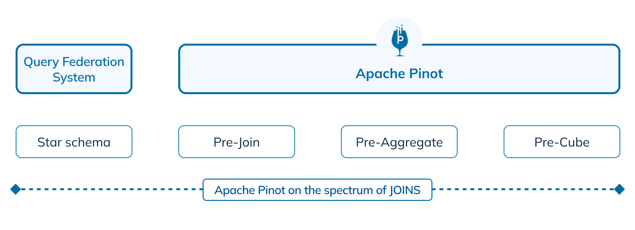
Figure 3: The data joining spectrum and support in Apache Pinot

Apache Pinot’s multi-stage query engine 

In May of 2022, we introduced a multi-stage query engine in Pinot. Prior to the introduction of the multi-stage query engine, Pinot had just a single stage scatter-gather mechanism between brokers and servers for serving queries (read more about Pinot’s architecture here). This worked well for the typical analytical queries such as high-selectivity filters and low-cardinality aggregations. However, for queries that require data shuffling, such as JOIN operations, a lot of the computation needs to be performed on the Pinot broker, effectively making it the bottleneck.

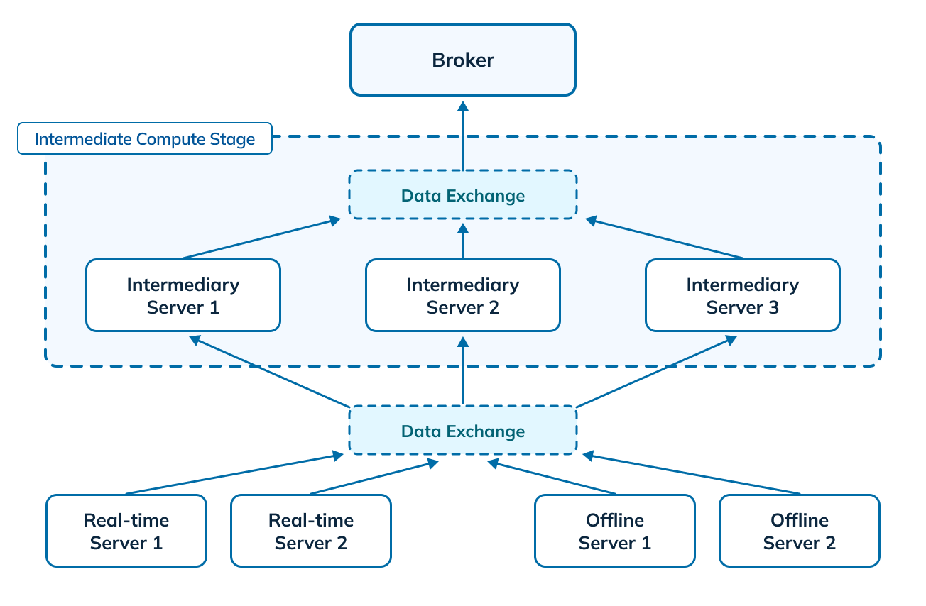
Figure 4: Multi-stage query engine in Apache Pinot

The multi-stage query engine is a generic processing framework, designed to handle complex multi-stage data processing. As part of the multi-stage execution model, we introduced a new intermediate compute stage in Pinot to handle the additional processing requirements and offload the computation from the brokers. The intermediate compute stage consists of a set of processing servers and a data exchange mechanism. We leverage the Pinot servers for the role of processing servers in the intermediate compute stage, but these can be assigned to any Pinot component. The data exchange service coordinates the transfer of the different sets of data to and from the processing servers. We also introduced a new query planner, which is designed to support full SQL semantics. 

With the multi-stage query engine, we had also released a preliminary version of JOINs, with limited functionality to target some specific use cases.  

JOINs support in Apache Pinot 1.0

With release 1.0, Apache Pinot now supports all join types - left, right, full, semi, anti, lateral and in-equi join. With this increased coverage of JOIN semantics, Pinot is now also SSB (Star Schema Benchmark) compatible. 

With native query-time JOINs in Pinot, we can now cover the entire spectrum of data joins, providing full coverage from user-facing analytics all the way up to ad hoc analytics. While query federation systems such as Trino are still necessary for joining datasets across data sources, the support of native JOINS in Pinot removes the dependence on these systems to perform joins solely within the scope of Pinot. 

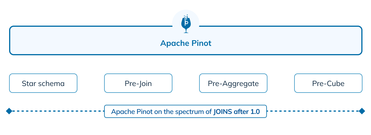
Figure 5: The data joining spectrum and support in Apache Pinot 1.0

When adding JOINs support, functional completeness of all JOIN semantics was just a small part of the story. We wanted to make sure that adding JOINs support doesn’t drop the performance of the system all the way to the band of star schema performance as shown in figure 2 above. Our users love the speed of Pinot, and rely on the sub-second latencies and high throughput for building user-facing real-time analytics applications. In this release, we focused heavily on improving the performance and the ability to execute JOINs optimally at scale, helping us serve JOINs with sub-seconds latency!

Basics of JOINs

Before we dive into the JOIN algorithms and optimizations in Apache Pinot, let’s set some context by taking a brief look at what a JOIN entails.

A JOIN involves stitching two tables — the left table and the right table — to generate a unified view, based on a related column between them. For example, below is a basic INNER JOIN query on two tables, one containing user transactions and another containing promotions shown to the users, to show the spending for every userID.

SELECT 
  p.userID, t.spending_val

FROM promotion AS p JOIN transaction AS t 
  ON p.userID = t.userID

WHERE
  p.promotion_val > 10
  AND t.transaction_type IN ('CASH', 'CREDIT')  
  AND t.transaction_epoch >= p.promotion_start_epoch
  AND t.transaction_epoch < p.promotion_end_epoch 

Query 1: A basic JOIN query on left table “promotion” with right table “transaction” with JOIN on column “userID”, and filters on “promotion_val”, “promotion_start_epoch”, “promotion_end_epoch”, “transation_type” and “transaction_epoch”

JOIN algorithms

There are three ways to execute a join. Let’s take the example of joining the two tables, the left table (L) and the right table (R). 

• Broadcast join: All data post filtering from the right table (R), is shipped to all nodes (N) of the left table (effective data moved R * N). This works well for cases when the filtered data being shipped is small and the number of nodes is also small. But query latency increases proportionately as the size of R increases or the number of nodes N increases. 

• Shuffle distributed hash join: After applying filters, data from both sides (L and R) is hashed on the join key and shipped to an independent shuffle stage (effective data moved L + R). This scales well even if the size of data on either side increases. Plus, the performance is unaffected by the number of nodes on either side.

• Lookup join: Right table must be pre-loaded (replicated) on all nodes of left table. This can only work for very small right hand datasets. 

  

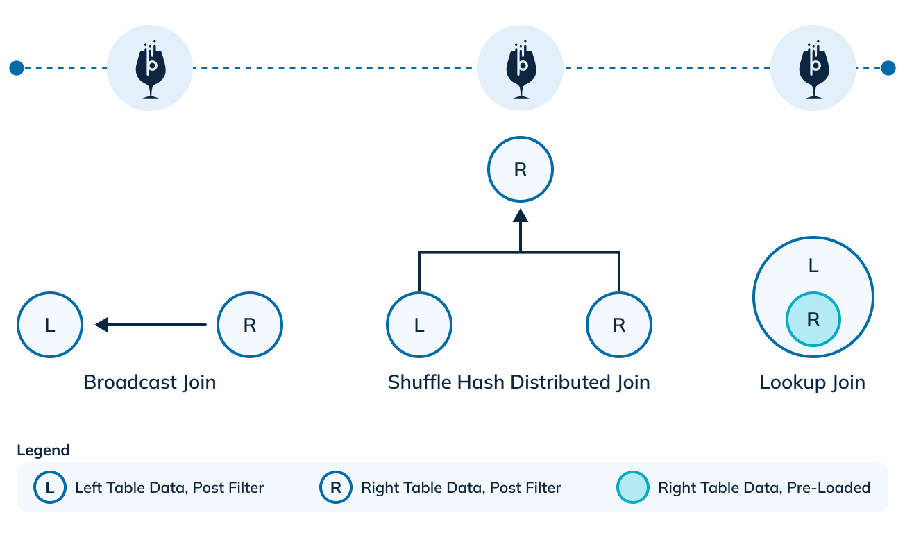
Figure 6: Join algorithms

With the 1.0 release, Apache Pinot can support all three types of join strategies. Amongst the other similar systems, lookup join is the only join algorithm that Druid can execute and broadcast join is the only algorithm supported by ClickHouse.

Stages of a JOIN

When implementing a shuffle hash distributed join in a database, it is typically tackled in at least two steps:

Figure 7: Basic pieces when executing a shuffle hash distributed JOIN

Scan

Data in each of the tables involved in the JOIN are scanned. If any filters are associated with the table, those are applied during the scan. Then, the data in the tables is partitioned using the columns in the join key. Finally, the partitions are forwarded to the shuffle phase.

Shuffle

After the scan, the data partitions for the same key from both tables are sent to the same server. This allows these intermediate servers to join the records from left and right, before sending the results to the next query processing stages. 

When implementing JOINs in Pinot, the design principle we followed was to do the least amount of work wherever possible by reducing the overhead of scans and minimizing the data shuffle. In each stage we have focused on adding optimizations to reduce the amount of such work done.

JOINs optimization strategies in Apache Pinot

Let’s walk through the JOIN optimizations strategies added in Apache Pinot.

Optimizations to reduce the amount of work done

Consider the below query, that joins two tables on multiple columns, with filters on both tables and grouping across tables:

SELECT 
  SUM(p.promotion_val - t.spending_val) AS net_val,
  count(*) AS total_cnt, 
  p.userID, t.spending_type

-- joining multiple keys
FROM promotion AS p JOIN transaction AS t 
  ON p.userID = t.userID AND p.region = t.region

WHERE p.promotion_val > 10 
  AND t.transaction_type IN ('CASH', 'CREDIT')
  AND t.transaction_epoch > 1693526400
  AND p.promotion_start_epoch > 1693526400

-- grouping across tables
GROUP BY 
  p.userID, t.spending_type

ORDER BY 
  1, 2

Query 2: A query joining table “promotion” and table “transaction”, on columns “userID” and “region”, with two filter predicates on each of the individual tables, grouping across the tables on “userID” and “spending_type” to compute aggregations 

Indexing and pruning

We make use of Pinot's rich set of indexes and pruning techniques to reduce the amount of work done when applying filters, thus speeding up query processing on the individual tables. We also use star-tree index – which serves as a filter as well as aggregation optimization – allowing us to push down and efficiently execute GROUP BY on the individual tables. 

Query 2 will be automatically rewritten as follows, so that we can push down the predicates and GROUP BY past the JOIN, to the individual tables:

WITH tmpP AS (
  SELECT 
    userID, region, 
-- pre-aggregation of values needed for the join later
    SUM(promotion_val) AS total_promo_val, COUNT(*) AS total_promo_cnt
  FROM promotion

-- push-down predicates restricted to a single table
  WHERE promotion_val > 10 
    AND promotion_start_epoch > 1693526400
    
-- star tree index used to speed up the group-by 
  GROUP BY userID, region
),

tmpT AS (
  SELECT 
    userID, region, spending_type,
-- pre-aggregation of values needed for the join later 
    SUM(transaction_val) AS total_trans_val, COUNT(*) AS total_trans_cnt
  FROM transaction

-- push-down predicates restricted to a single table
  WHERE t.transaction_type IN ('CASH', 'CREDIT')
    AND t.transaction_epoch > 1693526400

-- star tree index used to speed up the group-by
  GROUP BY userID, region, spending_type
)

SELECT 
  SUM(total_promo_val) - SUM(total_trans_val) AS net_val, 
  SUM(total_promo_cnt * total_trans_cnt) AS total_count
  p.userID, t.spending_type

FROM tmpP AS p JOIN tmpT AS t 
  ON p.userID = t.userID AND p.region = t.region
GROUP BY 
  p.userID, t.spending_type
ORDER BY 
  1, 2

Query 3: Query 2 rewritten to pushdown predicates for “promotion” on “promotion_val” and “promotion_start_epoch” and for “transaction” on “transaction_type” and “transaction_epoch, and to pushdown GROUP BY on “userID” and “spending_type”

These optimizations help in reducing the overhead of scanning and aggregations, as well as reducing the amount of data shuffled, all of which directly helps with improving query latency as well as throughput. 

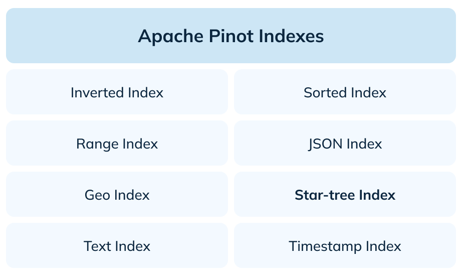
Figure 8: Indexes in Apache Pinot

Pinot’s indexes also allow us to effectively utilize optimizations such as dynamic filtering. As the name suggests, dynamic filtering is a performance optimization that dynamically remodels the query as a filter clause on one table, using the results of the other table. This optimization can significantly improve the performance of JOIN queries, especially in the case of high-selectivity joins. 

Here’s an example query, that can be rewritten to make use of dynamic filtering:

SELECT 
  p.promotion_type, AVG(p.promotion_val)
FROM promotion AS p JOIN user AS u ON p.userID = u.userID
WHERE
  u.life_time_val < 200
  AND p.promotion_val > 10
GROUP BY
  p.promotion_type

Query 4: A JOIN query on tables “promotion” and “user”, on column “userID” . Let’s assume that the filter on “user” for “life_time_val < 200”  is highly selective, and matches only a few users. If run as is, although a filter will be applied on “user”, the “promotion” table will undergo a full scan and transfer all table data to shuffle.

-- userID is the primary key of `user` table, thus justifies the semi-join optimization

SELECT
  promotion_type, AVG(promotion_val)
FROM promotion
WHERE 
  promotion_val > 10
  AND userID IN (
    SELECT userID FROM user 
    WHERE life_time_val < 200
)
GROUP BY
  promotion_type

Query 5: With dynamic filtering in Pinot, the query 4 can be rewritten as a filter clause on “promotion.userID” using results from “user.userID”.

Data layout

The data layout of the tables involved in join can have a huge impact on the performance of the join, particularly in the data shuffle stage. The aspects of data layout we will consider here are partitioning and co-location.

Terminology

Partitioning

Partitioning involves creating physical partitions of the table data, based on the join key. This is done upfront when the data is ingested into the database. Partitions of any given key are physically present on the same server, for a given table.

Co-location

Co-location involves placing the partitions for any given key on the same physical servers. This is done across all the tables involved in the join.

To illustrate how these layouts help in reducing the overall shuffle work, let's take an example where we have two tables to join, table L and table R.

Random layout

The most non optimal case is when data is neither partitioned, nor co-located. As you can see here, the scan stage has to create the data partitions. Data for a particular key could be dispersed over all the servers. To bring data for the same key onto the same server for the join, almost all of the post-filter data from both tables will need to be transferred, making the data transferred equal to (L + R).

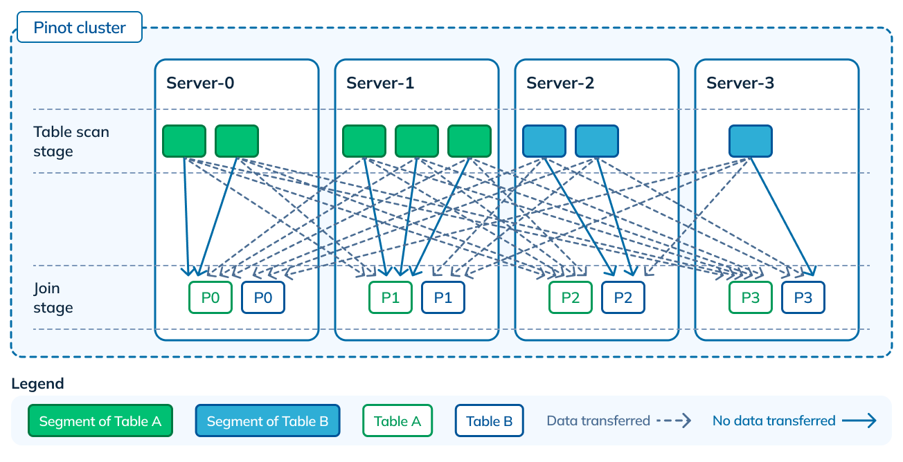
Figure 9: No partitioning in either of the tables, hence no co-location

Partitioned but not co-located

Now let’s take the case where data is partitioned, such that data for a given partition is guaranteed to be on a single node, for both tables. However there is no co-location, and hence no guarantees that data from the same partition across the tables will be on the same server. This is still better than the previous layout, because shuffle will only involve bringing partitions from one table to where the partitions of the other table exist, making the transfer overhead equal to (R). 

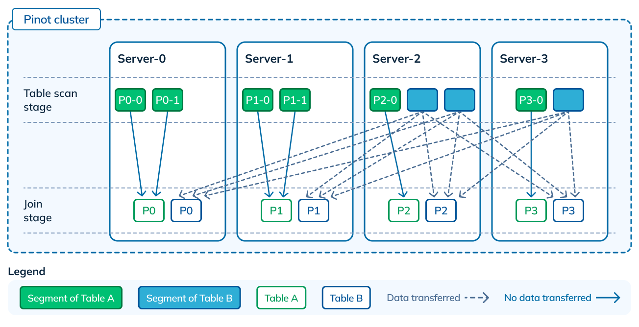
Figure 10: Partitioning in Table A, but no co-location with Table B

Partitioned and co-located

Now let’s take this one step further, where both tables are partitioned and the partitions created are co-located. This is highly optimal, as the data shuffled becomes 0. The servers have all the data for a particular key, and can directly start executing the join.

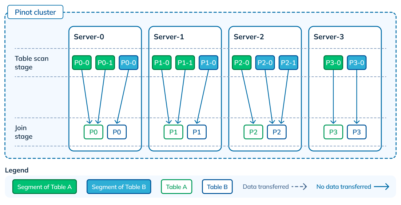
Figure 11: Both tables partitioned, as well as partitions co-located

In Pinot, you can run a JOIN on data with any of these layouts. However, if a favorable data layout is available, Pinot can take advantage of it to run a more efficient join. Although this sounds obvious, not every OLAP database has the ability to adapt based on the data layout, and often end up doing more work than is required resulting in higher query latencies. 

Query hints

While some optimizations are native to Pinot, or designed to kick in by default, the more advanced ones are provided as query hints. These query hints are designed to give finer control to the users to either reduce the operator overhead or bring down the data shuffle. 

For instance, in the example from above involving tables “promotion” and “user”, if there are a lot more promotions than user signups and “user” table is small enough to fit in memory, or if “promotion” table is partitioned by “userID”, it makes sense to broadcast “user” table to “promotion” table for better performance.

SELECT /*+ joinOptions(join_strategy='dynamic_broadcast') */ 
  promotion_type, promotion_val
FROM promotion
WHERE 
  promotion_val > 10
  AND userID IN (
    SELECT userID FROM user 
    WHERE channel IN (‘REFERRAL’, ‘MOBILE_AD’)
)
GROUP BY
  promotion_type

Query 6: Passing a hint to the query to use dynamic broadcast

In the future, we will automate these query hints, so the user won’t have to manually set them in the query.

Performance

Performance benchmarking is highly dependent on use case, query pattern, and dataset. We recommend you evaluate query performance on your datasets. But just to give an idea of the ballpark numbers to expect, here’s some results we saw on 10TB data placed on 16 servers with 4 cores each. The query was a LEFT JOIN query, with a filter on the left table, and an aggregation GROUP BY with ORDER BY. The number of records in the left table were 6 billion, with 1 billion records post-filter, and the number of records in the right table were 130 million.

SELECT 
  count(*), t1.col, t2.col 
FROM 
  table1 t1 LEFT JOIN table2 t2 ON 

  t1._guid = t2._guid 
  
WHERE
  t1._orgid = “<value>”
GROUP BY 
  t1.col
ORDER BY 
  t1.col desc

Query 7: LEFT JOIN with filter, aggregation and GROUP BY ORDER BY

Here’s the optimizations we applied with each new iteration, and the effect it had on the query latency:

As you can see, with every optimization we applied, we were able to systematically bring the latency down, all the way to sub-seconds. We significantly reduced the architectural complexity compared to the alternate solution, which consisted of using three systems (Elasticsearch, Redshift and Presto) plus a custom query router.

Conclusion

With the availability of JOINs in Apache Pinot, we cover the entire spectrum of JOINs and have unlocked a whole new range of applications and use cases. With optimizations for using data layout and predicate pushdown, we are able to run smarter JOINs, achieving better performance than what other OLAP databases can accomplish.

Figure 12: Handling star schema in Apache Pinot via native JOINs, compared to other techniques in the spectrum of JOINs

A huge shout out to all the Pinot committers and contributors involved in making this amazing feat possible! You can try out JOINs in Apache Pinot, by downloading the 1.0 release. We welcome you to join our community Slack channel, to learn more about this feature. You can also meet the team at an upcoming meetup, or keep in touch with us on Twitter at @ApachePinot.

We also invite you to try out StarTree Cloud – a fully managed experience for deploying and operating Apache Pinot. Sign up for a 30-day free trial of our Public SaaS offering or order it directly from AWS or Azure marketplaces. We’d love to hear from you in our Slack community.

Apache Pinot