StarTree-Index Impact on Query Performance

StarTree-Index is a specialized index in Apache Pinot™. that dynamically builds a tree structure to maintain aggregates for a group of dimensions. With star-tree Index, the query latency becomes a function of just a tree traversal with computational complexity of log( n ) .

This comprehensive blog explains in depth how the star-tree Index differs from traditional materialized views (MVs). In particular, read the section Star-Tree Index: Pinot’s intelligent materialized view . Particularly this one key passage:

Star-Tree Index: Pinot’s Intelligent Materialized View:

The star-tree index provides an intelligent way to build materialized views within Pinot. Traditional MVs work by fully materializing the computation for each source record that matches the specified predicates. Although useful, this can result in non-trivial storage overhead. On the other hand, the star-tree index allows us to partially materialize the computations and provide the ability to tune the space-time tradeoff by providing a configurable threshold between pre-aggregation and data scans.

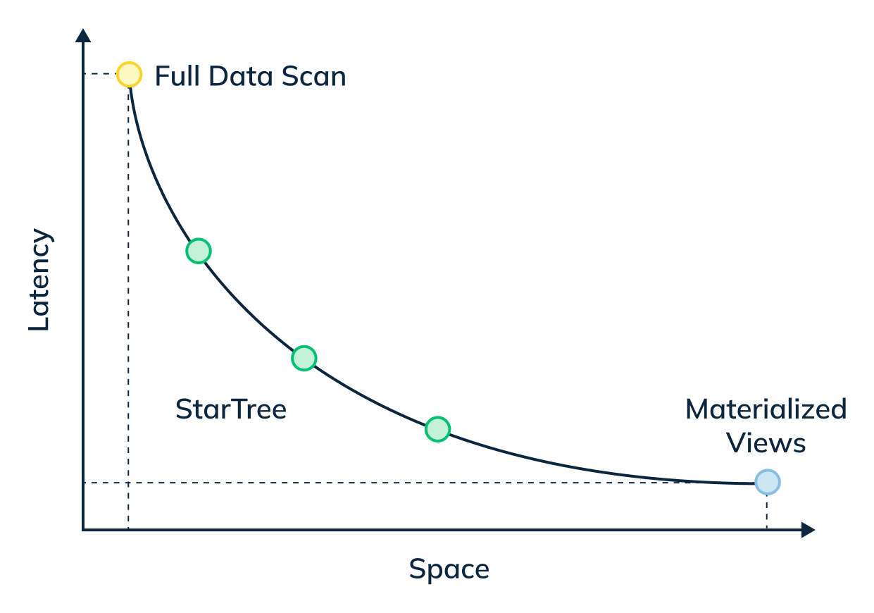
In this three-part blog series, we will compare and contrast query performance of a star-tree index with an inverted index, something that most of the OLAP databases end up using for such queries.

In this first part, we will showcase how a star-tree index brought down standalone query latency on a sizable dataset of ~633M records from 1,513ms to 4ms! — nearly 380x faster.

1. The Dataset:

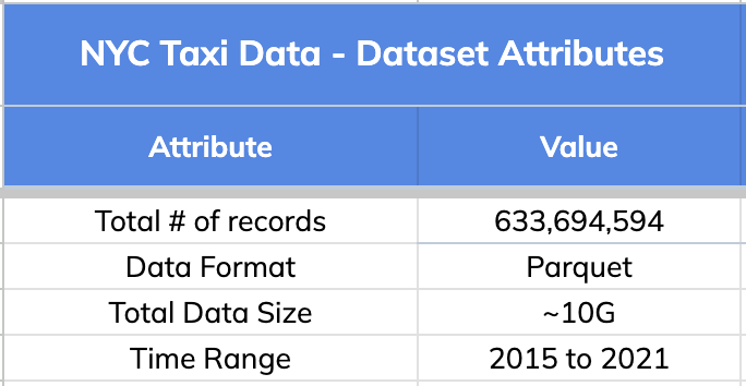
We used New York City Taxi Data for this comparison. Original source: here. Below are the high level details about this dataset.

Schema:

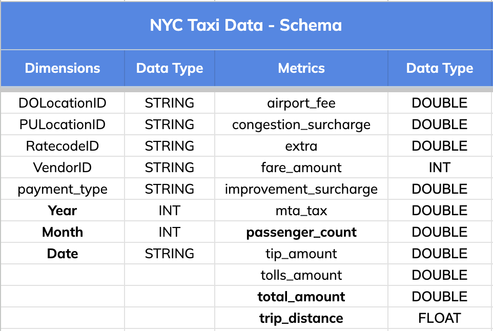
The dataset has 8 dimension fields and 11 metric columns as listed below.

2. Query Pattern

The query pattern involved slicing and dicing the data (GROUPING) BY various dimensions (Date, Month and Year), aggregating different metrics (total trips, distance and passengers count) and FILTERING BY a time range that could go as wide as 1 year.

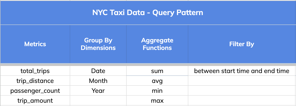
Note: A key thing to note is that a single star-tree index covers a wide range of OLAP queries that comprise the dimensions, metrics and aggregate functions specified in it.

Star-Tree Index Config:

To support the various query patterns specified above, we defined the following star-tree index.

"starTreeIndexConfigs": [  { 
 "dimensionsSplitOrder": [ 
 "dropoff_date_str", 
 "dropoff_month", 
 "dropoff_year" 
 ], 
 "skipStarNodeCreationForDimensions": [], 
 "functionColumnPairs": [ 
 "COUNT__*", 
 "SUM__passenger_count", 
 "SUM__total_amount", 
 "SUM__trip_distance", 
 "AVG__passenger_count", 
 "AVG__total_amount", 
 "AVG__trip_distance", 
 "MIN__passenger_count", 
 "MIN__total_amount", 
 "MIN__trip_distance", 
 "MAX__passenger_count", 
 "MAX__total_amount", 
 "MAX__trip_distance" 
 ], 
 "maxLeafRecords": 10000 
 } 
 ]

This one star-tree index can get us insights to questions such as:

How many trips were completed in a given day, month or year?
How many passengers traveled in a given day, month or year?
What is the daily / monthly / annual average trip revenue?
What is the daily / monthly / annual average trip revenue, trip duration and distance traveled?
What is the daily / monthly / annual breakdown of total number of trips, total distance traveled and total revenue generated in 2015?
And many more…

We will use one such variant query for this illustration:

What is the total number of trips, total distance traveled and total revenue generated by day in 2015?

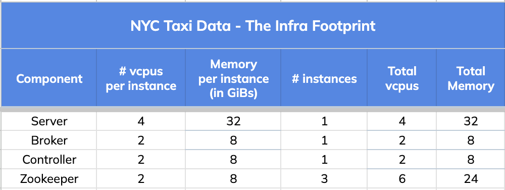
3. The Infra Footprint

We used a very small infrastructure footprint for this comparison test.

4. Query Results and Stats

Iteration #1: w/o any Apache Pinot optimizations:

First, we ran the query without any optimizations offered in Apache Pinot.

-- Iteration #1: w/o optimizations > 120s  
SELECT 
 toDateTime(tpep_dropoff_datetime/1000, 'yyyy-MM-dd') "Date", 
 count(*) "Total # of Trips", 
 sum(trip_distance) "Total distance traveled", 
 sum(passenger_count) "Total # of Passengers", 
 sum(total_amount) "Total Revenue" 
FROM 
 nyc_taxi_demo 
WHERE 
 "Date" BETWEEN '2015-01-01' AND '2015-12-31' 
GROUP BY 
 "Date" 
ORDER BY 
 "Date" ASC 
limit 1000

This was a wide time range query (365 days). It required scanning across ~146M out of ~633M documents. In addition, it involved performing an expensive ToDateTime transformation on the tpep_dropoff_datetime entry in each of those ~146M documents during query time .

Result: The query took 131,425 milliseconds (~131.4s; ~2m 11s) to complete.

Iteration #2: w/ Inverted Index

In this iteration, we used a derived column – dropoff_date_str – which performed the ToDateTime transformation for every record during ingestion time . Since the cardinality of this derived column was much lower (granularity was at Day level instead of milliseconds), this enabled us to use an inverted index on this column.

-- Iteration #2: w/ Ingestion Time Transformation SELECT 
 dropoff_date_str "Date", 
 count(*) "Total # of Trips", 
 sum(trip_distance) "Total distance traveled", 
 sum(passenger_count) "Total # of Passengers", 
 sum(total_amount) "Total Revenue" 
FROM 
 nyc_taxi_demo 
WHERE 
 "Date" BETWEEN '2015-01-01' AND '2015-12-31' 
GROUP BY 
 "Date" 
ORDER BY 
 "Date" ASC 
limit 1000 
option(useStarTree=false, timeoutMs=20000)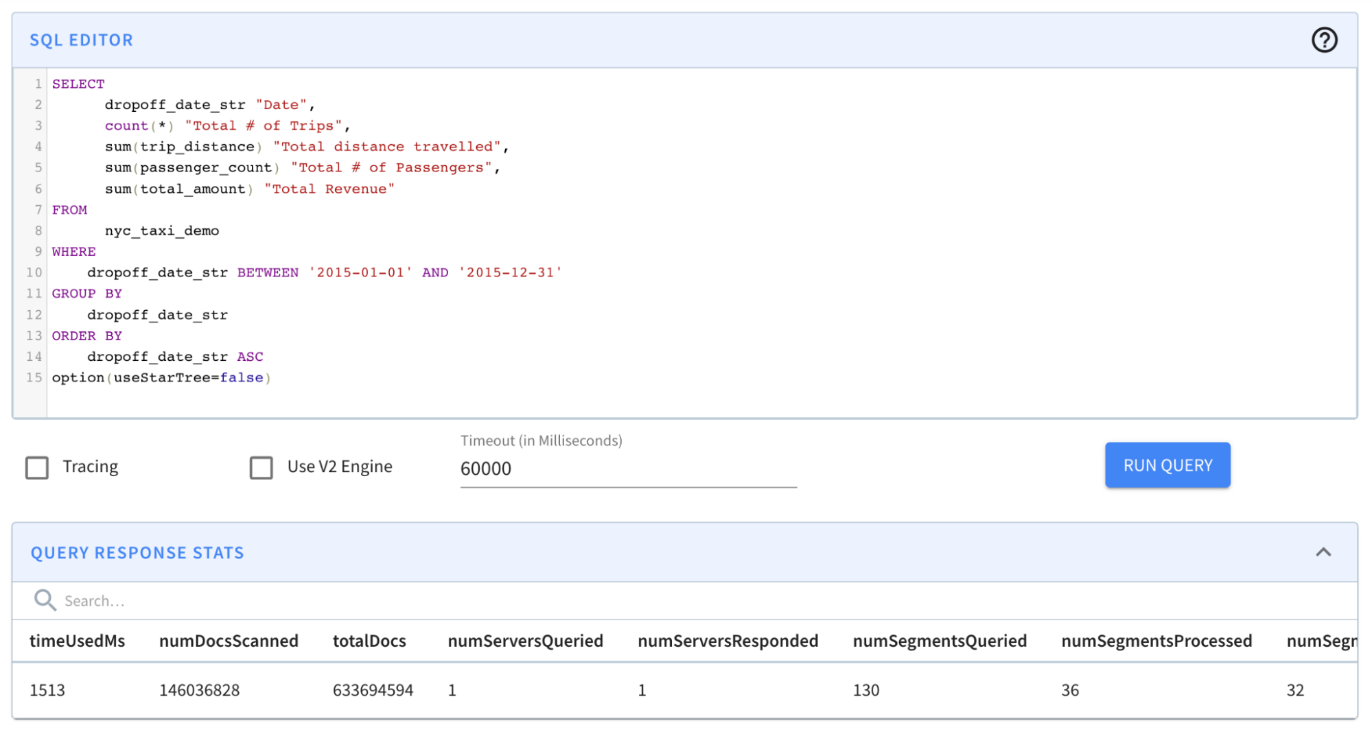

Result: The query completed in 1,513 milliseconds. (~1.5s); from ~131s to ~1.5s was a BIG improvement. However, results still took more than a second — which is a relatively long time for an OLAP database, especially if it is faced with multiple concurrent queries.

Iteration #3: w/ Star-Tree Index:

In this iteration, we ran the same query with star-tree index enabled.

-- Iteration #3: w/ Ingestion Time Transformation + StarTree Index SELECT 
 dropoff_date_str "Date", 
 count(*) "Total # of Trips", 
 sum(trip_distance) "Total distance traveled", 
 sum(passenger_count) "Total # of Passengers", 
 sum(total_amount) "Total Revenue" 
FROM 
 nyc_taxi_demo 
WHERE 
 "Date" BETWEEN '2015-01-01' AND '2015-12-31' 
GROUP BY 
 "Date" 
ORDER BY 
 "Date" ASC 
limit 1000 
option(useStarTree=true)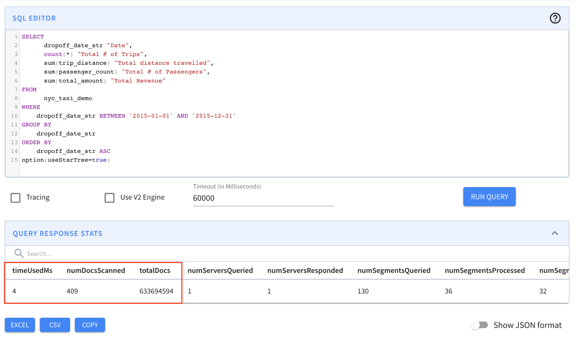

Result: The query completed in 4 milliseconds! Notice in particular that the numDocsScanned came down from ~146M to 409!

Comparison:

Let’s take a closer look at the query response stats across all three iterations to understand the “how” part of this magic of indexing in Apache Pinot.

The dataset has 633,694,594 records (documents) spread across 130 segments.
Query Stats:
1. w/o any index optimizations (Iteration #1), the query scanned ALL 633,694,594 records (check numEntriesScannedInFilter) during processing. Also, numEntriesScannedPostFilter was 584,147,312 (numDocsScanned = ~146M). All 130 segments were processed which was very inefficient.
2. w/ Inverted Index (Iteration #2), numEntriesScannedInFilter was 0; numEntriesScannedPostFilter was 584,147,312 (numDocsScanned = ~146M) which meant that the query selectivity was low (the query had to scan a lot of records during post filter phase; about 92% of overall records). This is an indication of when a star-tree index could help.
3. w/ Star-tree Index (Iteration #3), numEntriesScannedInFilter was 0; numEntriesScannedPostFilter was only 2,045 (numDocsScanned = 409). The star-tree index helped improve query performance tremendously by providing high query selectivity .

5. Impact Summary:

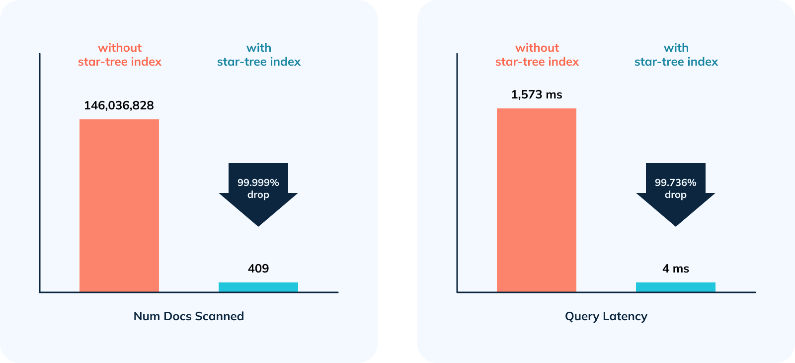
356,968x improvement (or 99.999% drop) in num docs scanned from ~146M to 409 .
378.5x improvement (~99.736% drop) in query latency from 1,513 ms to 4 ms .

Key Benefits of the Star-Tree Index:

User controllable: Tune space vs. time overhead
Flexible: create any number of indexes. The right index is chosen based on the query structure.
Transparent: Unlike traditional MVs, users don’t need to know about the existence of a star-tree index. The same query will be accelerated with a star-tree index in place.
Dynamic: Very easy to generate a new index at any point of time.
Disk IO is the most expensive operation in query processing. Latency is linear to the number of disk reads a query has to perform. Star-Tree Index brings the number of disk reads down exponentially.
- In this example, star-tree Index reduced the disk reads by 99.999% from ~584 Million entries (~146 Million documents or records) in case of an inverted index to 2,045 entries (409 documents or records). Query latency came down from 1,513 ms to 4 ms!

In part 2 of this series, we will perform throughput tests to measure the impact of star-tree index under high load.

Star-Tree Indexes in Apache Pinot - Part 1: Understanding the Impact on Query Performance