Geospatial Indexing in Apache Pinot

It’s been over 18 months since geospatial indexes were added to Apache Pinot™, giving you the ability to retrieve data based on geographic location—a common requirement in many analytics use cases. Using geospatial queries in combination with time series queries in Pinot, you can perform complex spatiotemporal analysis, such as analyzing changes in weather patterns over time or tracking the movement of objects, vehicles, or people. Pinot's support for geospatial data indexing means fast and efficient querying of large-scale, location-based datasets distributed across multiple nodes.

In that time, more indexing functionality has been added, so I wanted to take an opportunity to have a look at the current state of things.

What is geospatial indexing?

Geospatial indexing is a technique used in database management systems to store and retrieve spatial data based on its geographic location. It involves creating an index that allows for efficient querying of location-based data, such as latitude and longitude coordinates or geographical shapes.

Geospatial indexing organizes spatial data in such a way that enables fast and accurate retrieval of data based on its proximity to a specific location or geographic region. This indexing can be used to answer queries such as "What are the restaurants with a 30-minute delivery window to my current location?" or "What are the boundaries of this specific city or state?"

Geospatial indexing is commonly used in geographic information systems (GIS), mapping applications, and location-based services such as ride-sharing apps, social media platforms, and navigation tools. It plays a crucial role in spatial data analysis, spatial data visualization, and decision-making processes.

How do geospatial indexes work in Apache Pinot?

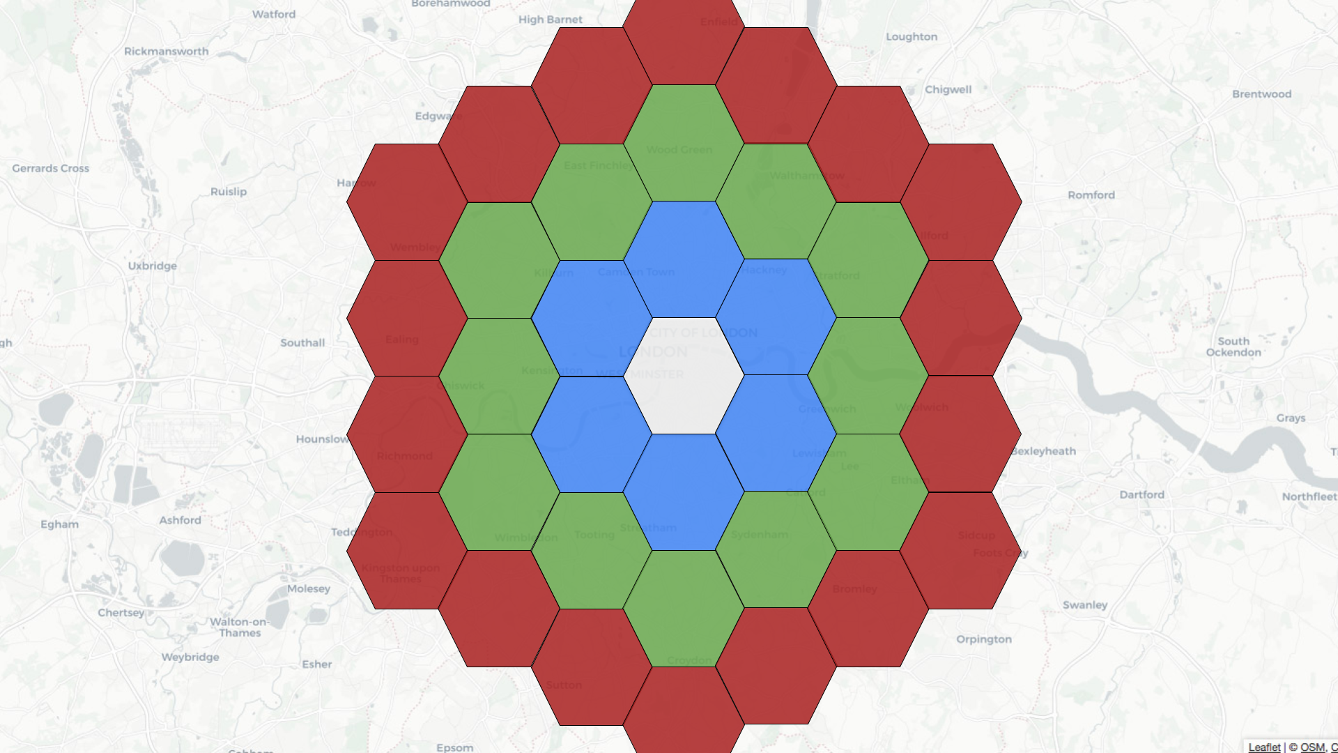
We can index points using H3, an open source library that originated at Uber. This library provides hexagon-based hierarchical gridding. Indexing a point means that the point is translated to a geoId, which corresponds to a hexagon. Its neighbors in H3 can be approximated by a ring of hexagons. Direct neighbors have a distance of 1, their neighbors are at a distance of 2, and so on.

For example, if the central hexagon covers the Westminster area of central London, neighbors at distance 1 are colored blue, those at distance 2 are in green, and those at distance 3 are in red.

Let’s learn how to use geospatial indexing with help from a dataset that captures the latest location of trains moving around the UK. We’re streaming this data into a trains topic in Apache Kafka®. Here’s one message from this stream:

kcat -C  -b localhost:9092 -t trains -c1| jq


{
  "trainCompany": "CrossCountry",
  "atocCode": "XC",
  "lat": 50.692726,
  "lon": -3.5040767,
  "ts": "2023-03-09 10:57:11.1678359431",
  "trainId": "202303096771054"
}

We’re going to ingest this data into Pinot, so let’s create a schema:

{
    "schemaName": "trains",
    "dimensionFieldSpecs": [
      {"name": "trainCompany", "dataType": "STRING"},
      {"name": "trainId", "dataType": "STRING"},
      {"name": "atocCode", "dataType": "STRING"},
      {"name": "point", "dataType": "BYTES"}
    ],
    "dateTimeFieldSpecs": [
      {
        "name": "ts",
        "dataType": "TIMESTAMP",
        "format": "1:MILLISECONDS:EPOCH",
        "granularity": "1:MILLISECONDS"
      }
    ]
}

The point column will store a point object that represents the current location of a train. We’ll see how that column gets populated from our table config, as shown below:

{
    "tableName": "trains",
    "tableType": "REALTIME",
    "segmentsConfig": {
      "timeColumnName": "ts",
      "schemaName": "trains",
      "replication": "1",
      "replicasPerPartition": "1"
    },
    "fieldConfigList": [{
        "name": "point",
        "encodingType":"RAW",
        "indexType":"H3",
        "properties": {"resolutions": "7"}
    }],
    "tableIndexConfig": {
      "loadMode": "MMAP",
      "noDictionaryColumns": ["point"],
      "streamConfigs": {
        "streamType": "kafka",
        "stream.kafka.topic.name": "trains",
        "stream.kafka.broker.list": "kafka-geospatial:9093",
        "stream.kafka.consumer.type": "lowlevel",
        "stream.kafka.consumer.prop.auto.offset.reset": "smallest",
        "stream.kafka.consumer.factory.class.name": "org.apache.pinot.plugin.stream.kafka20.KafkaConsumerFactory",
        "stream.kafka.decoder.class.name": "org.apache.pinot.plugin.stream.kafka.KafkaJSONMessageDecoder"
      }
    },
    "ingestionConfig": {
      "transformConfigs": [
        {
          "columnName": "point",
          "transformFunction": "STPoint(lon, lat, 1)"
        }
      ]
    },
    "tenants": {},
    "metadata": {}
}

The point column is populated by the following function under transformConfigs:

STPoint(lon, lat, 1)

In earlier versions of Pinot, you’d need to ensure that the schema included lat and lon columns, but that no longer applies. 

We define the geospatial index on the point column under fieldConfigList. We can configure what H3 calls resolutions, which defines the size of a hexagon and their number. A resolution of 7 means that there will be 98,825,150 hexagons, each covering an area of 5.16 km². We also need to add the geospatial column to tableIndexConfig.noDictionaryColumns.

We can go ahead and create that table using the AddTable command and Pinot will automatically start ingesting data from Kafka.

When is the geospatial index used?

The geospatial index is used when a WHERE clause in a query calls the StDistance, StWithin, or StContains functions.

ST_Distance

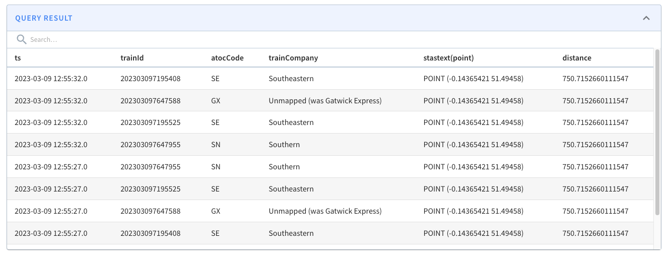
Let’s say we want to find all the trains within a 10 km radius of Westminster. We could write a query to answer this question using the STDistance function. The query might look like this:

select ts, trainId, atocCode, trainCompany, ST_AsText(point),
       STDistance(
         point, 
         toSphericalGeography(ST_GeomFromText('POINT (-0.13624 51.499507)'))) 
  AS distance
from trains 
WHERE distance < 10000
ORDER BY distance, ts DESC
limit 10	

These results from running the query would follow:

Let’s now go into a bit more detail about what happens when we run the query.

The 10 km radius covers the area inside the white circle on the diagram below:

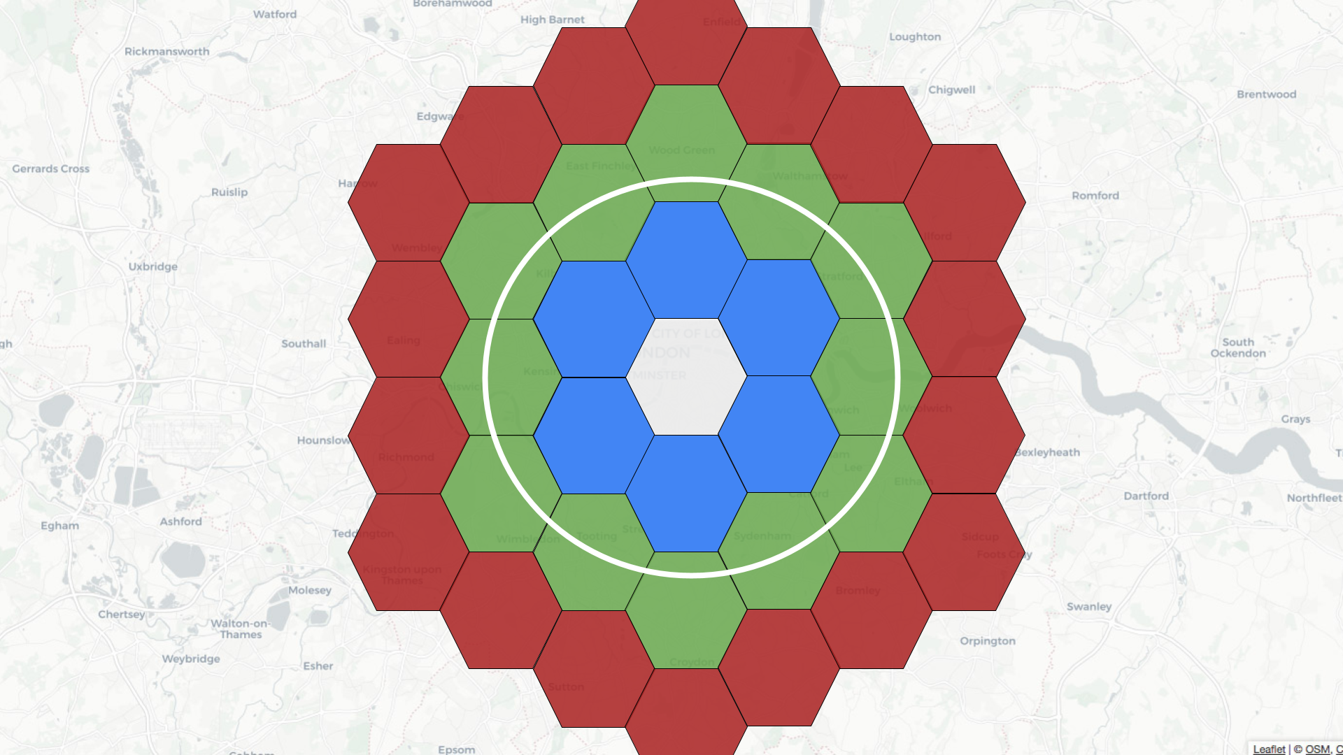
Pinot’s query planner will first translate the distance of 10 km into a number of rings, in this case, two. It will then find all the hexagons located two rings away from the white one. Some of these hexagons will fit completely inside the white circle, and some will overlap with the circle.

If a hexagon fully fits, then we can get all the records inside this hexagon and return them. For those that partially fit, we’ll need to apply the distance predicate before working out which records to return.

ST_Within/ST_Contains

Let’s say that rather than specifying a distance, we instead want to draw a polygon and find the trains that fit inside that polygon. We could use either the ST_Within or ST_Contains functions to answer this question.

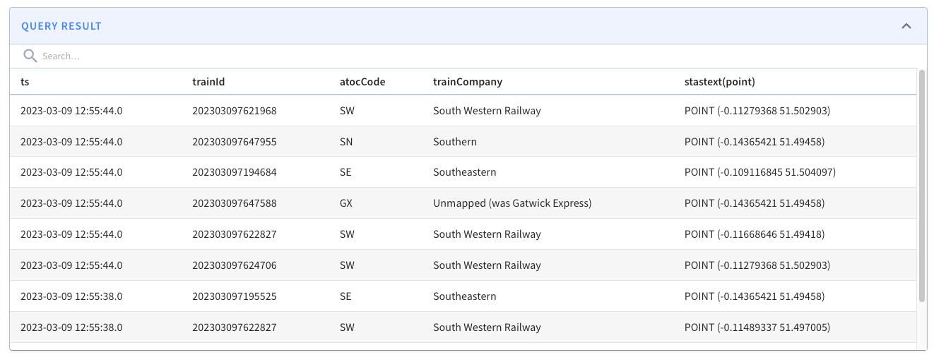
The query might look like this:

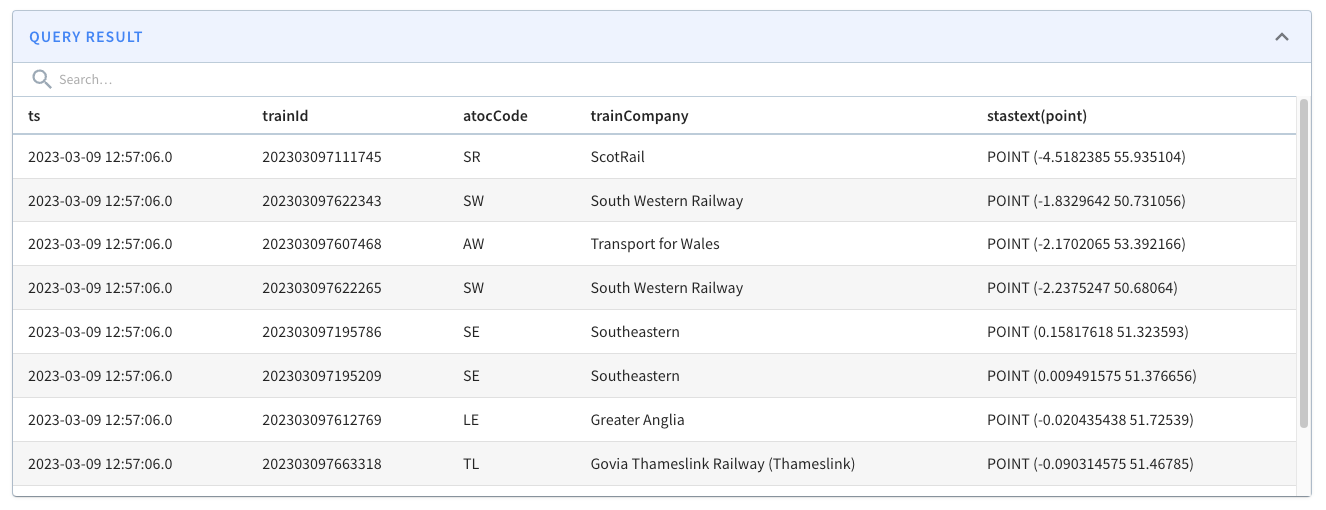
select ts, trainId, atocCode, trainCompany, ST_AsText(point)
from trains 
WHERE StWithin(
      point, 
      toSphericalGeography(ST_GeomFromText('POLYGON((
        -0.1296371966600418 51.508053828550544,
        -0.1538461446762085 51.497007194317064,
        -0.13032652437686923 51.488276935884414,
        -0.10458670556545259 51.497003019756846,
        -0.10864421725273131 51.50817152245844,
        -0.1296371966600418 51.508053828550544))'))) = 1
ORDER BY ts DESC
limit 10

The results from running the query are shown below:

If we change the query to show trains outside of a central London polygon, we’d see the following results:

So what’s actually happening when we run this query? 

The polygon covers the area inside the white shape as shown below:

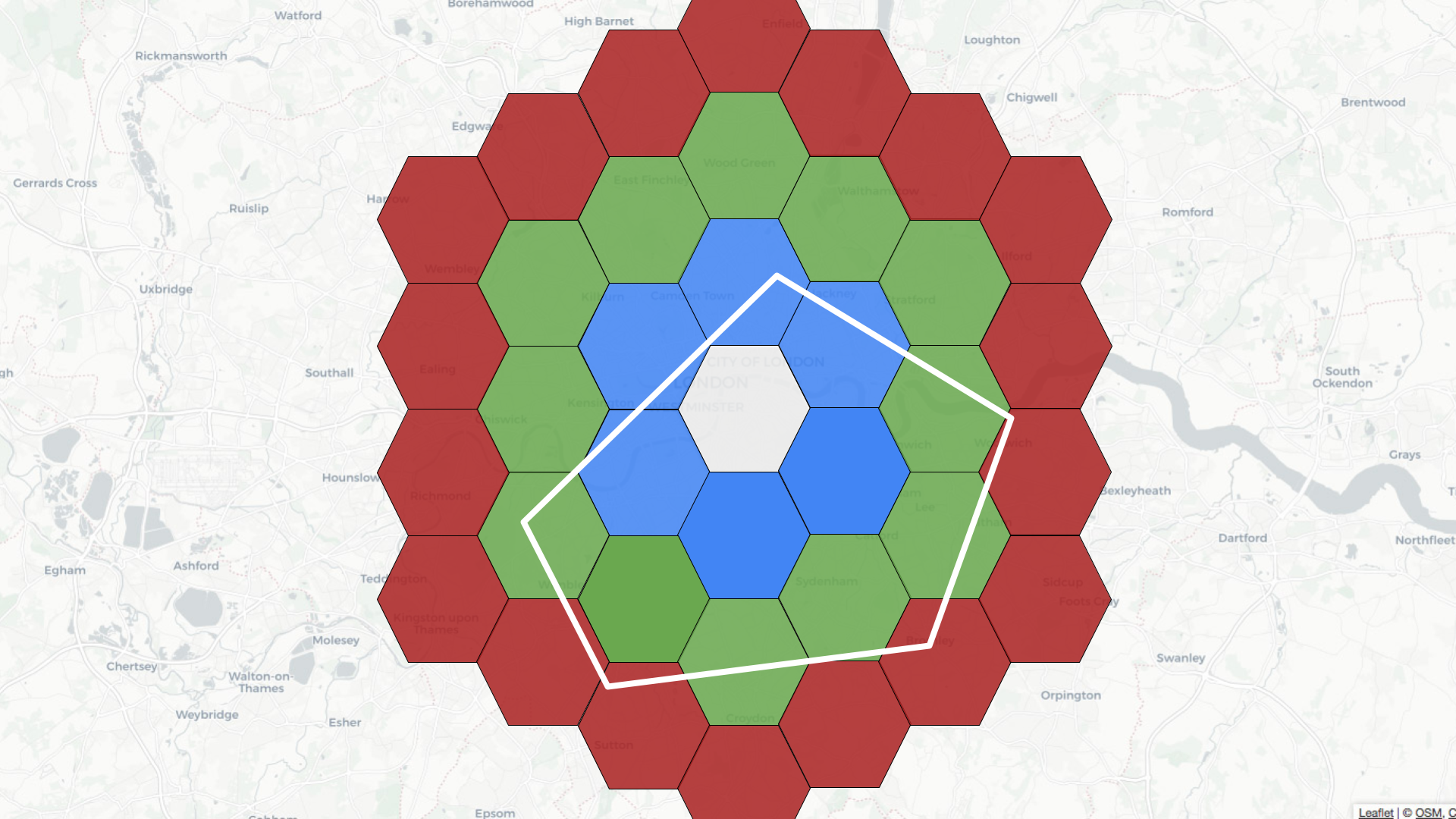
Pinot’s query planner will first find all the coordinates on the exterior of the polygon. It will then find the hexagons that fit within that geofence. Those hexagons get added to the potential cells list. 

The query planner then takes each of those hexagons and checks whether they fit completely inside the original polygon. If they do, then they get added to the fully contained cells list. If we have any cells in both lists, we remove them from the potential cells list.

Next, we find the records for the fully contained cells list and those for the potential cells list. 

If we are finding records that fit inside the polygon, we return those in the fully contained list and apply the STWithin/StContains predicate to work out which records to return from the potential list.

If we are finding records outside the polygon, we will create a new fully contained list, which will actually contain the records that are outside the polygon. This list contains all of the records in the database except the ones in the potential list and those in the initial fully contained list. 

This one was a bit tricky for me to get my head around, so let’s just quickly go through an example. Imagine that we store 10 records in our database and our potential and fully contained lists hold the following values:

potential = [0,1,2,3]
fullyContained = [4,5,6]

First, compute newFullyContained to find all the records not in potential:

newFullyContained = [4,5,6,7,8,9]

Then we can remove the values in fullyContained, which gives us:

newFullyContained = [7,8,9]

We will return all the records in newFullyContained and apply the STWithin or StContains predicate to work out which records to return from the potential list.

How do you know the index usage?

We can write queries that use STDistance, STWithin, and STContains without using a geospatial index, but if we’ve got one defined, we’ll want to get the peace of mind of its actual use.

You can check by prefixing a query with EXPLAIN PLAN FOR, which will return a list of the operators in the query plan. 

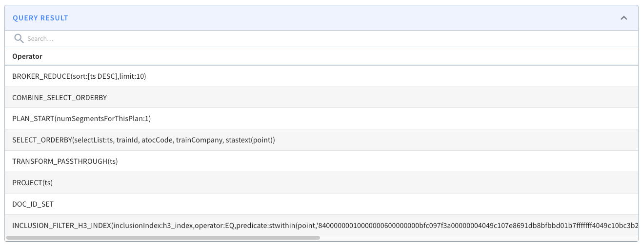
If our query uses STDistance, we should expect to see the ​​FILTER_H3_INDEX operator. If it uses STWithin or STContains, we should expect to see the INCLUSION_FILTER_H3_INDEX operator.

See this example query plan:

The StarTree Developer Hub contains a geospatial indexing guide that goes through this in more detail.

Summary

I hope you found this blog post useful and now understand how geospatial indexes work and when to use them in Apache Pinot.

Give them a try, and let us know how you get on! If you want to use, or are already using geospatial queries in Apache Pinot, we’d love to hear how — feel free to contact us and tell us more! To help get you started, sign up for a free trial of fully managed Apache Pinot. And if you run into any technical questions, feel free to find me on the StarTree Community Slack.

Apache Pinot