4 Elements of the Modern Data Architecture for Real-Time Analytics

In today’s fast-paced business world, data is most valuable in real-time or near real-time. To support this continuous flow of data, companies need a modernized data architecture designed for real-time analytics — not just a traditional data architecture modified to support near real-time or real-time data sources. While there are many variations, a general underlying architectural pattern has emerged across organizations and industries. You may already have one or more of these components running in your own data architecture.
In this blog, I’ll cover 4 key components of a modern data architecture with native support for real-time analytics:
- Omni-channel data sources
- Transactional systems
- Data streaming / pipelining layer
- OLAP / analytical systems
Let’s start by looking at a simplified sketch of the next-generation data analytics architecture.
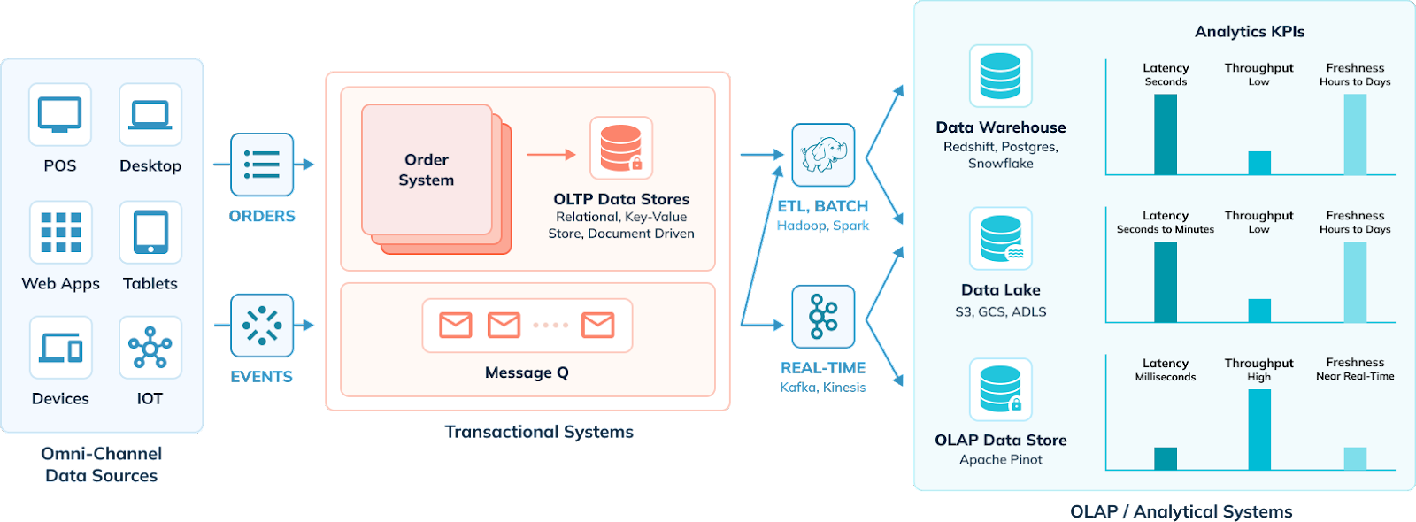
1. Omni-channel data sources
On the left side, there are different data generators. These are the web applications, mobile apps, point-of-sale systems in retail stores, smart IoT devices, tablets. The data generators, operating independently or with human input, generate operational data on a day-to-day basis.
2. Transactional systems (aka OLTP)
All the operational data gets stored in transactional (OLTP) data stores. These data stores are either relational SQL systems (MySQL, Oracle, Postgres, etc.), or NoSQL systems of various types, including document-driven (MongoDB, CouchDB, etc.), key-value stores (DynamoDB, Redis, etc.), wide column (Cassandra, ScyllaDB), or graph (Tigergraph, Neo4j, etc.).
The transactional data stores are designed to support write-heavy use cases, as many applications write to these data stores at any point in time. They are mostly row-oriented data stores, with each write operation corresponding to creating or updating a row-based record. IO is the most expensive operation when it comes to database read/write performance. In order to support high write throughput (QPS), the schema in transactional SQL systems is normalized to eliminate redundancy and avoid multiple disk writes per request. However, many NoSQL systems ingest denormalized data, which bloats the amount of information stored on disk, but also allows for fast writes.
3. Data streaming / pipelining
Data from original sources and stored in transactional systems needs to reach analytical systems. Originally and traditionally these processes were batch-oriented Extract, Transform, and Load (ETL) tools.
However, in more recent years users have implemented real-time data streaming systems such as Apache Kafka (and Kafka-compatible services), Apache Pulsar, Amazon Kinesis and so on. Data can also be transformed prior to ingestion into an analytical database using stream processing systems like Apache Flink. For example, normalized data from OLTP SQL systems may be pre-joined (denormalized) prior to ingestion into a real-time OLAP system.
Historical data can even be brought in from object stores, or data warehouses using ETL data pipelines, and combined with real-time data streams to create a complete view of information. This is known as a hybrid table.
4. Analytical systems (aka OLAP)
All the operational data from various data sources and transactional systems is eventually loaded into the analytical systems. The purpose behind this is to centralize all the operational data to cross reference and derive meaningful insights geared towards improving organizational efficiencies and monitoring business KPIs.
Online Analytical Processing (OLAP) systems are divided into a number of sub-types:
- Real-time analytics (real-time OLAP) systems seek to provide answers in the span of seconds or subsecond times. Because the priority is speed and volume of query processing, data tends to be used in denormalized forms.
- Data warehouses are focused on being a structured repository of corporate data, cleaned and processed. Quality of data is a key consideration. Ingestion into a data warehouse requires stringent quality checks, governance, and normalization across all data sources, so there is one single coherent view of a customer. Query performance is a far lower priority.
- Data lakes are similar to data warehouses, yet store unprocessed, raw data. The primary consideration is scalability (and affordability of storage). Again, timely query performance is a far lower priority.
- Data lakehouses are architecturally designed to combine the best attributes of a data lake and a data warehouse. Like both of those systems, data scalability and quality are the priorities, not raw performance.
The paradigm in analytical systems is very different from that in transactional systems. The use cases are predominantly read-heavy. Writes are generally done once at time of initial ingestion. However, some real-time OLAP systems can also deal with upserts — a combination operation that performs an insert if a record does not exist, and an update to a record if it already exists.
Similar to NoSQL transactional (OLTP) systems, the schema in real-time OLAP systems is most often denormalized or flattened; a storage tradeoff is made by introducing data redundancy in lieu of faster read performance. However, even though data schemas may be denormalized, many real-time analytics systems still use the same query semantics of SQL. As well, some real-time OLAP systems can maintain multiple tables in a star schema and perform query-time JOINs, like OLTP SQL databases.
Analytical systems are powered by three powerful technologies, as described in the following section.
In any next-generation data analytics architecture, you will notice all three technologies being present, each powering different sets of use cases. Having said that, these technologies are converging and the decision to choose one for your specific use case should be made based on the analytics KPIs described at the far right of the architecture diagram.
D ata warehouses
Data warehouses have been around for many decades.
- Data format: Data warehouses are relational in nature; data is structured.
- Schema: In data warehouses, schema is fixed and predefined; they support schema-on-write.
- Use cases: Data warehouses are designed for internal analytics use cases such as dashboarding and reporting. In data warehouses, compute and storage are tied together, which helps in achieving faster query SLAs. The query SLA range data warehouses can achieve is in seconds to minutes.
- Analytics KPIs:

- Query latency range is in seconds to minutes.
- Query throughout is fairly low (under 1). We are talking about a few internal users running queries spread throughout the day.
- Data freshness is in hours to days. The data is ETLed from transactional systems using periodic jobs — typically once nightly; or at best hourly throughout the day during low activity windows.
Data lakes (object stores)
With the advent of newer data formats, which traditional data warehouses could not support natively, data lake technology came to life. Object stores data lakes have compute and storage completely decoupled. The data is stored in object stores such as Amazon S3, where the cost of storage is very cheap (compared to block storage attached to the VM). Big data compute engines like Hive, Spark, and Presto are used for serving advanced analytics.
- Data format: Designed for storing data in its purest form; structured, semi-structured, or unstructured .
- Schema: Flexible schema, schema-on-read.
- Use cases: Internal analytics; data science, machine learning, and advanced analytics use cases.
- Analytics KPIs:

- For analytical queries, data lakes provide query latencies in minutes to hours. Compared to data warehouses, data lakes make performance tradeoffs in lieu of cost and flexibility in terms of support for different data formats.
- Query throughput is low (typically under 10).
- Data freshness is in hours to days. The data is ETLed from transactional systems using periodic jobs — typically once nightly; or at best hourly throughout the day during low activity windows.
A nalytical data stores
With the advent of user-facing applications that serve insights and metrics to end users, sub-second latencies became quintessentially important and that’s where analytical data stores came to life. The data in these systems is stored in columnar format; richer indexes are added to meet the query latency SLAs in milliseconds.
In addition, new use cases that demanded putting metrics directly in front of the external user arose. The scale and throughput support needed for these external user-facing applications was unprecedentedly high as compared to internal user-facing analytics use cases. And lastly, with the advent of real-time streaming sources, data freshness became another important KPI to chase after for businesses.
- Data format: Columnar storage; typically analytical data stores support structured data; Apache Pinot natively supports storing semi-structured data.
- Schema: Fixed schema; schema-on-write.
- Use cases: Designed for user-facing analytics use cases that demand ultra-low latency (sub-second) and data freshness of near real-time.
- Analytics KPIs:

- Query latency range is in milliseconds.
- Query throughput is low (internal user facing) to high (external user facing).
- Data Freshness is in near real-time. The data needs to be made available for querying as soon as possible after arriving on the real-time stream.
Introducing Apache Pinot
Apache Pinot is an analytical data store that is designed to support a wide spectrum of analytical use cases; marquee use cases powered in production today by Apache Pinot are LinkedIn’s “Who Viewed My Profile” and UberEats “Restaurant Manager.”
These use cases require support for:
- Latency: Ultra-low query latencies (in milliseconds) as there is an end user waiting for a response on the other side
- Throughput: An extremely high read throughput (hundreds of thousands of Read QPS)
- Data freshness: Data freshness of near real-time (in a few seconds)
Apache Pinot provides that ultra-low latency for analytical queries under high read throughput and near real-time data freshness. Additionally, Apache Pinot natively supports upserts, which helps use cases such as UberEats Restaurants Managers to keep track of changing order status in real-time.
Introducing StarTree Cloud
StarTree is an enterprise-ready, cloud-native, and fully managed Apache Pinot platform. With the StarTree Cloud platform, customers get an option to have tightly coupled (Local SSDs), loosely coupled (Remote SSDs/EBS), or completely decoupled storage from compute (Tiered Storage) for their Pinot deployment. Depending on the KPI requirements of their use cases, the customers make that tradeoff between cost and performance; and achieve blazing fast, sub-second latencies for their use cases.
Book a demo with our experts to see StarTree Cloud in action. You can also get started with fully managed Apache Pinot by signing up for our 30-day free trial.