
Latency is only half the result
Stripe runs a time-series aggregation system on Apache Pinot at 150K events per second and 20K QPS, with p99 query latency of 21 ms and p99.9 of 63 ms. Across Stripe’s broader Pinot deployment, its largest cluster holds roughly 3 PB of data, and Pinot powered the Black Friday–Cyber Monday transactional dashboard that tracked more than 300 million transactions representing over $18.6 billion in transaction volume.
These production numbers are cited to make the serving problem concrete, not as a limit on Pinot’s query throughput, data scale, or achievable latency.
They lead to the question this article explores: what does the system have to do on every request to keep latency that low as data volume and concurrency grow?
The other half of the performance result is how much query-time work and serving capacity the architecture needs to keep that latency stable under sustained concurrency.
Two analytical databases can return the same query in 50 milliseconds and still require very different amounts of work. One may touch hundreds of megabytes, involve several compute nodes, issue many storage reads, and consume substantial CPU. Another may identify a much smaller candidate set through routing and indexes and return the same result with a much smaller resource footprint.
At hundreds or thousands of queries per second, that difference becomes a capacity problem. But higher concurrency is only one way the trade-off surfaces. Growth in data, query diversity, or the amount of work that survives each access path can expose the same issue at much lower QPS when tail latency has to stay fixed.
Two systems: Same latency, very different serving work
Consider two illustrative queries that return the same result set in 50 milliseconds:
| Query A | Query B | |
|---|---|---|
| Latency | 50 ms | 50 ms |
| Data touched | 800 MB | 8 MB |
| CPU consumed | 1.2 CPU-sec | 0.08 CPU-sec |
| Storage activity | High | Low |
| Workers involved | 8 | 3 |
| Result rows | 100 | 100 |
At 500 QPS, Query A represents roughly 400 GB/sec of logical data processing and 600 CPU-seconds of work per wall-clock second, versus 4 GB/sec and 40 CPU-seconds for Query B. That CPU work is equivalent to roughly 600 versus 40 continuously busy cores, a 15× difference in compute demand, before accounting for other system overhead.
Both are still “50 ms” queries, but they require very different amounts of system work to produce that latency.
Same query. Different amounts of work reach execution.
To see where that difference comes from, start with the work required to narrow a selective query before general execution begins. The rest of this article follows that path: what the system must do to discover the relevant data, what reaches execution, how that work translates into serving capacity, and how to measure it in a production-style POC.
How a selective query gets narrowed: PRUNE → FIND → READ
For a selective ClickHouse Cloud query, it helps to separate three kinds of work:
- PRUNE eliminates partitions and parts that cannot match.
- FIND analyzes the applicable indexes to identify candidate granules, up to about 8,192 rows each by default; adaptive granularity can make granules smaller for wider rows.
- READ retrieves and processes the surviving data through the cache/storage hierarchy.
ClickHouse Cloud’s SharedMergeTree architecture stores native table data in shared object storage rather than tying it to fixed physical shards. Compute replicas can therefore access the same logical dataset, while each query still has to determine which parts and granules are relevant before reading them.
For a SharedMergeTree query, partition and part elimination happen first. Primary-index analysis narrows the candidate granules. Secondary skip indexes can be evaluated up front or incrementally alongside data reads using streaming secondary indexes; in either path, they determine which granules can be skipped. The surviving granules are then read through the cache/storage hierarchy and processed by the execution engine. When the relevant index, mark, or data state is already resident in cache, that work can be considerably cheaper, but working-set size and locality still determine how much state must be fetched.
Pinot makes a different serving choice. Segment ownership, routing state, and persistent indexes are established before the request arrives. The Broker routes the query to the relevant segments; each Server evaluates the indexes on the segments it owns to narrow the candidate documents, then reads and processes the surviving data locally.
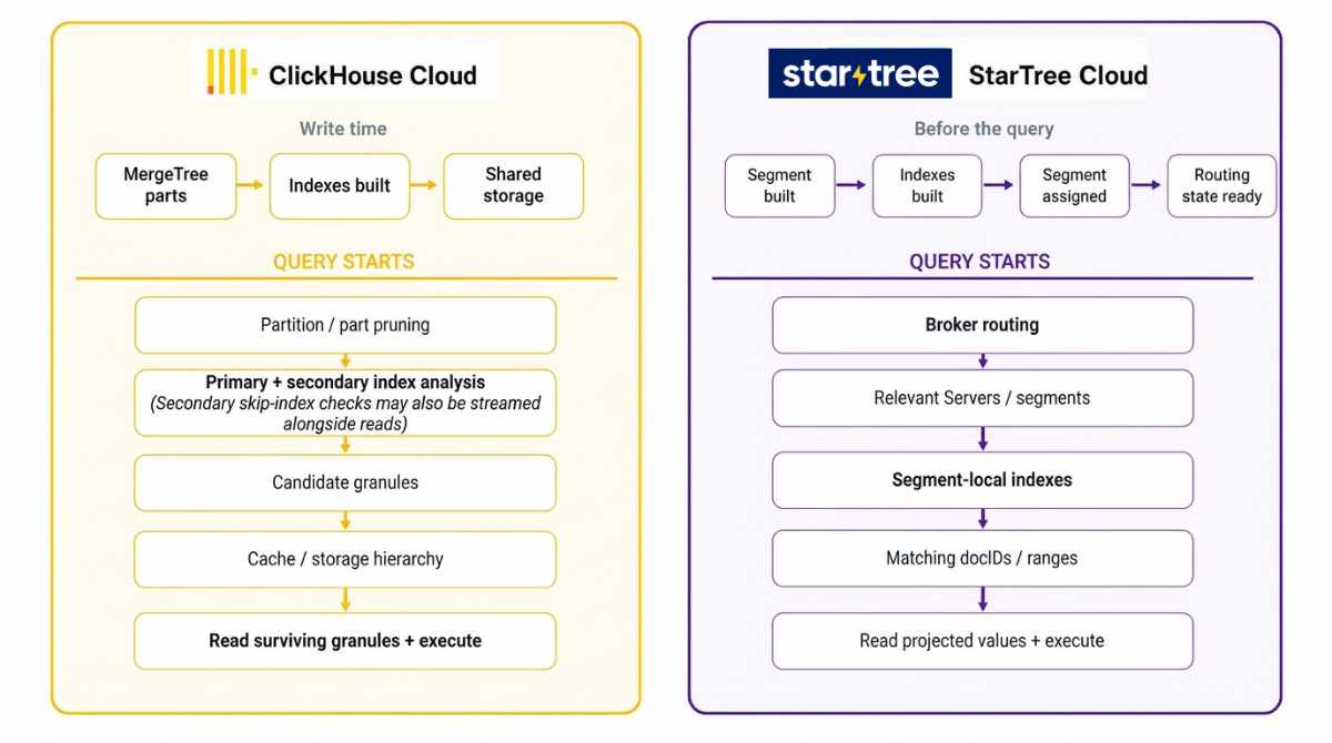
The easiest way to understand why that matters is with a query that returns almost nothing.
A five-row query can still require substantial lookup work
Here is the same customer lookup from the animation at a larger illustrative scale. Consider a table whose primary sort order is optimized around event time:
SELECT customer_id, amount
FROM events
WHERE event_time >= now() - INTERVAL 7 DAY
  AND customer_id = 734521
Because event_time aligns with the table’s physical ordering, the sparse primary index can efficiently narrow the request to the relevant seven-day range, but customer_id presents a different problem because it is not correlated with that order. For the illustration below, assume the seven-day range leaves 4,800 candidate granules, roughly 39 million rows of granularity at 8,192 rows per granule. A Bloom-filter data-skipping index on customer_id narrows those to 12 surviving granules. That is a substantial reduction, but those 12 granules still represent roughly 98K rows of granularity before the five matching rows are resolved.
This illustrates both the strength and the constraint of ClickHouse’s primary access path. When queries align with the table’s sort order, the sparse primary index can eliminate most granules very cheaply. But that sort order is part of the physical layout; it does not change as new query patterns arrive. Supporting those patterns therefore requires additional access structures, such as secondary indexes or projections, rather than a different primary ordering for each query. A projection can provide an alternative physical layout, but it is another structure that must be maintained.
Pinot can also use physical sorting as an optimization, but predicates on other dimensions can use independent indexes without reorganizing the segment around each one. Both systems therefore build access structures ahead of query time. The difference in this example is granularity: ClickHouse’s primary and most skip-index paths prune parts and granules, while Pinot indexes such as the inverted index can resolve a predicate to individual document IDs.
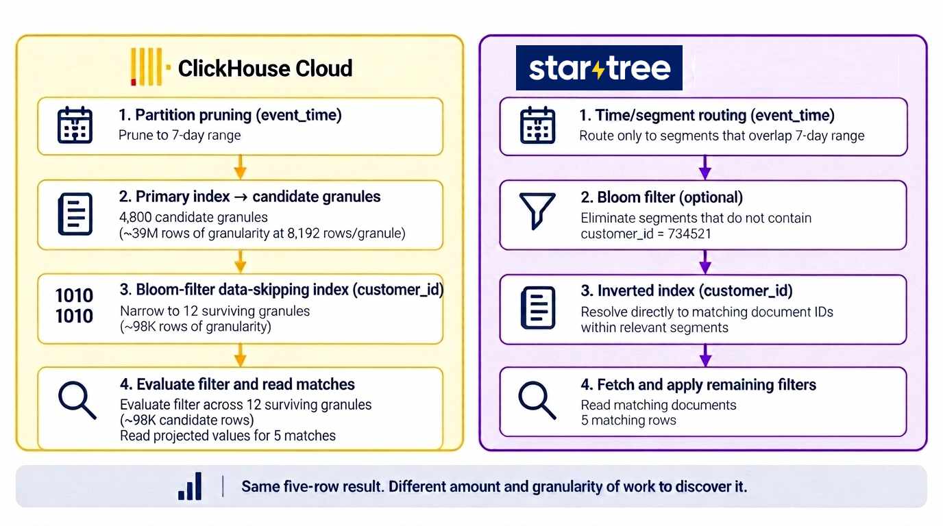
Pinot resolves the same five-row query differently
Assume customer_id has an inverted index and, optionally, a Bloom filter. As the illustration above shows, the Broker first routes the query to segments that overlap the requested time range. A Bloom filter can then eliminate segments that definitely do not contain customer_id = 734521. For the segments that remain, the inverted index resolves the equality predicate directly to the matching document IDs. If additional filtering is required inside the boundary segments, Pinot can apply another index or evaluate the predicate against the much smaller candidate document set.
ClickHouse can still reduce the cost of processing those surviving granules with mechanisms such as PREWHERE: filter columns are evaluated first, so other projected columns need only be read for rows that pass the filter. But PREWHERE does not change the candidate set produced by the data-skipping path: the customer_id predicate still has to be evaluated against the rows in those 12 surviving granules before the five matches are known.
That example isolates candidate granularity on one query. Production adds another dimension: as part count, index footprint, and query diversity grow, the work required just to decide what should be read can itself become material.
When FIND itself becomes a scaling problem
We normally think of distributed query execution as spreading expensive processing across machines: reading data, filtering rows, aggregating results, or joining large inputs. In ClickHouse Cloud, the work involved in figuring out which granules should be read in the first place can also become large enough to distribute.
With SharedMergeTree, authoritative table data lives in shared storage rather than being tied to fixed replicas. Each candidate part still has primary-index data, mark files, and any applicable secondary indexes. Primary-index analysis happens up front; secondary skip-index checks can be evaluated up front or streamed alongside data reads. When a large index footprint is analyzed up front, that work can consume meaningful memory and I/O before matching rows are read.
ClickHouse Cloud’s index-analysis cost also depends on cache state. If the relevant primary-index, mark, or secondary-index data is already in cache, that analysis can be considerably cheaper. A cold or newly added replica may need to retrieve that state from lower cache tiers or shared object storage before or during analysis.
ClickHouse can distribute different parts of this path. Distributed Index Analysis distributes the FIND stage, spreading upfront index analysis across replicas when enabled and activated. Parallel Replicas distributes the READ/execution stage across compute replicas.
ClickHouse’s own benchmark shows when index analysis becomes material
In ClickHouse’s 50-billion-row test, a table with roughly 17,000 parts and six million marks required about 8.5 seconds of local Bloom-filter index analysis. Distributing that work reduced the index-analysis time to roughly 1.1 seconds with 10 replicas and 0.65 seconds with 20 replicas. These are index-analysis times rather than end-to-end query latency, and index sharding remains a private-preview capability for SharedMergeTree tables.
ClickHouse built Distributed Index Analysis to address a specific limit in this path: adding replicas increases overall serving capacity, and Parallel Replicas can use those replicas to accelerate READ/execution for an individual query, but without index sharding the upfront FIND/index-analysis phase remains single-node. Distributed Index Analysis extends parallelism to that stage as well.
ClickHouse activates Distributed Index Analysis only once the problem is large enough to justify the coordination. The defaults, when the feature is enabled, are at least 10 parts and more than 1 GiB of combined uncompressed index data. ClickHouse describes the 1 GiB threshold as the point where analysis cost starts to shape query latency and per-replica working memory. These thresholds are activation defaults, not sizing guidance; the crossover depends on the candidate parts, index footprint, index types, and workload.
Index-analysis work grows with the workload
The 50-billion-row benchmark is an extreme illustration, but the mechanism is not limited to petabyte-scale deployments. As more applications use the same dataset, the service often accumulates more indexes and projections
A deployment may start with the base sort order and a few secondary indexes, then add Bloom filters, text search, vector indexes, projections, JSON indexes, or other structures as the query mix expands.
Each query uses only the structures relevant to it. Across the full workload, though, there is more index data to cache and more index-analysis work to support.
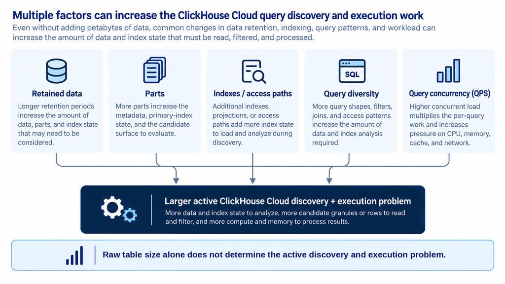
The crossover is therefore not determined by raw table size alone. Candidate parts, index footprint, cache state, and query mix determine how much discovery work sits on the request path. That matters because the problem can appear well before a petabyte-scale deployment: as applications add more query patterns, indexes, projections, and parts, FIND can become material even when the table itself is much smaller. If Distributed Index Analysis is not enabled or available, that work remains on one node, so preserving p95/p99 may require more per-replica CPU, memory, and I/O headroom instead.
In other words, this can become a production sizing problem long before it becomes a petabyte-scale data problem.
Pinot keeps index responsibility with segment ownership
Pinot also pays the cost of maintaining indexes, but query-time responsibility is organized differently. Segments and their persistent indexes are assigned to specific Servers before the request arrives. With replica-group routing, each Server therefore evaluates only the index state associated with the segments it owns, within one serving copy.
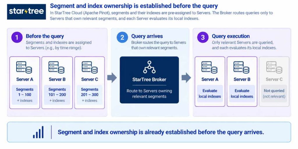
Growth can still require more Servers and segment capacity, but index-analysis responsibility remains tied to segment ownership rather than being repartitioned at query time.
Up to this point, the comparison has been about discovering the relevant rows. The production consequence is what survives that discovery and enters execution
What less query-time work buys you in production
At serving scale, the benefit of a selective access path extends beyond read latency. Every record filtered out early is one less record the system has to read, process, move across the network, aggregate, or keep in memory.
The same idea extends beyond row elimination to the physical cost of reading the rows that survive. We saw this clearly in a recent production-style StarTree POC over roughly 8 TB, sustaining 50 QPS while ingesting 15K events/sec, with multi-table joins, large time windows, group-bys, aggregations, and derived metrics. The application targets were p95 below 2 seconds and p99 below 5 seconds.
Physical layout matters in Pinot too. In this POC, a business dimension used in nearly every query was deliberately chosen as the sorted column. That improved locality, changing the physical access pattern from scattered, seek-heavy reads to fewer and more contiguous reads. Under load, the observed disk-read pattern improved by 3-5x even though the business query itself had not changed.
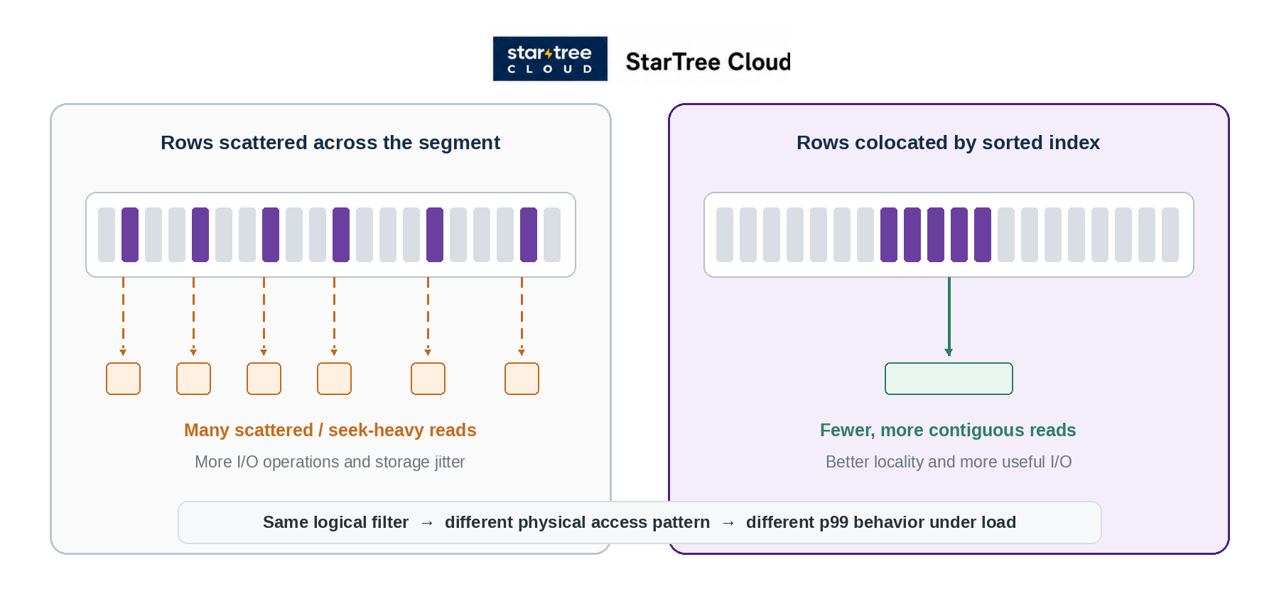
That sorted-column choice in this POC is therefore one locality optimization, not a requirement for every selective predicate.
Other dimensions can use independent access paths, including inverted, range, JSON, geospatial, sparse, and other indexes, without reorganizing the segment around each one. The broader principle is the same: eliminate irrelevant data early and make the surviving reads cheaper. Fewer surviving rows mean less data to read, decode, filter, move, and aggregate, while better locality makes more efficient use of the I/O that remains.
As QPS increases, those per-query differences multiply. In the POC above, Pinot tuning reduced the per-query work and helped bring application p95/p99 from roughly 6s/15s to 1.8s/3.6s. Native and vectorized execution can make the remaining work cheaper, but they cannot eliminate data that still has to be read, decoded, filtered, exchanged, or aggregated.
That POC shows the effect inside a mixed, production-style workload. A public benchmark gives us a cleaner version of the same question: when the data is already warm, how much CPU work does each request still create?
Reyden Benchmark: what drives CPU when the data is already warm?
Databricks originally demonstrated TPC-H Q6 at high concurrency using Reyden. ClickHouse then reconstructed the SF1 workload and published a more detailed response, including throughput and resource usage. StarTree subsequently reproduced the same basic Q6/SF1 fixed-parameter workload directly against an external Parquet table.
The query itself is simple: three filters followed by a SUM.
SELECT sum(l_extendedprice * l_discount) AS revenue
FROM lineitem
WHERE l_shipdate >= '1994-01-01'
  AND l_shipdate < '1995-01-01'
  AND l_discount BETWEEN 0.05 AND 0.07
  AND l_quantity < 24;Code language: PHP (php)
The interesting part is how small the dataset is. TPC-H SF1 is roughly a 1 GB benchmark dataset, and LINEITEM contains exactly 6,001,215 rows. At ClickHouse’s default 8,192-row granularity, that is only about 733 granule-equivalents for LINEITEM.
ClickHouse itself makes essentially the same point: SF1 is small enough to fit comfortably in memory, so once the benchmark is warm, this is primarily a test of how efficiently the engine uses CPU against cached data rather than a large-scale storage I/O test.
ClickHouse reports that a 30-vCPU, 120-GB node sustains about 420 QPS while keeping P90 below one second. Beyond that point, CPU becomes the limiting resource. Reading ClickHouse’s published multi-node curve, the 20-node, 600-vCPU configuration crosses the one-second P90 threshold at roughly 9,300 QPS.
Why does a small, memory-resident query still need that much compute?
Keeping the data in memory removes most storage latency. It does not remove the work the CPU still has to perform on every request: examine indexes and marks, access and decode column blocks, evaluate the filters, process the surviving values, calculate l_extendedprice * l_discount, and aggregate the result.
ClickHouse does not publish the exact table DDL or read_rows for this Reyden-response run, so its scan path cannot be stated as fact. But its published TPC-H LINEITEM layout is ordered by (l_orderkey, l_linenumber), while Q6 filters on l_shipdate, l_discount, and l_quantity. Only about 1.9% of rows qualify, yet those matches should be distributed throughout a table ordered by order key. At 8,192 rows per granule, that is roughly 156 qualifying rows per granule on average, leaving little opportunity for the primary sort order to eliminate whole granules.
Absent additional Q6-aligned skipping structures, the published layout therefore suggests that most granules would still reach the read-and-filter path. That provides a plausible explanation for the CPU-heavy execution profile: keeping the data warm removes much of the storage latency, but not the CPU and memory-bandwidth required to decode, filter, and aggregate a large candidate set.
ClickHouse points out that the benchmark could be improved further by tuning the number of threads, enabling the query cache, creating projections, and making other optimizations. Those suggestions connect directly to the earlier sections of this article.
Reducing the number of threads changes how CPU is shared across concurrent requests. A query cache can avoid executing the same query again when its result can be reused. A projection can give Q6 a physical layout that better matches its filters, allowing ClickHouse to eliminate more granules before execution.
That last option is also exactly the trade-off we have been discussing. The way to make the query cheaper is to reduce how much data reaches execution. Additional projections and indexes can do that, but they also add maintained access structures aligned to additional query patterns as the dataset and query mix grow. In ClickHouse Cloud, that brings its own operating trade-offs: more index state to maintain, a larger cache working set, and potentially more index-analysis work as the deployment grows.
StarTree took a different path on the same query.
StarTree’s follow-up benchmark took a different path. It queried a StarTree External Table backed directly by Parquet in object storage, using Range Indexes on l_shipdate, l_discount, and l_quantity.
We did not first convert the dataset into Pinot’s native segment format. For the SF1 run, we also did not use a query-result cache or Star-Tree preaggregation. ClickHouse’s test, in contrast, first loaded the Databricks TPC-H data into a ClickHouse table before running the workload.
The StarTree range indexes reduced 6,001,215 rows to 114,160 candidate documents before the main execution work began, roughly a 52.6x reduction.
With 12 StarTree Servers plus 12 Brokers, 240 serving vCPUs in total (242 including the shared Controller), the system served 11,996 QPS at 19.2 ms P90 with zero errors and stayed below one-second P90 through roughly 16,000 QPS.
At the same one-second P90 threshold, that is roughly 16,000 QPS on 242 total vCPUs for StarTree versus 9,300 QPS on 600 vCPUs for ClickHouse. Both are warm-state serving results. With storage latency less dominant, the amount of data reaching execution and the CPU work performed per request become central to the capacity difference.
ClickHouse appears extremely efficient at processing hot rows. In the StarTree run, the Range Indexes eliminated most rows before the main execution work began.
Processing rows faster matters. Processing far fewer rows can matter even more.
That is why latency alone is not enough. Measure how many rows reach execution, how much CPU each request consumes, how many replicas participate, and how much total serving capacity is required to keep the target p99 as QPS grows.
What happens when too many rows still match?
Most of the examples so far reduce the number of rows entering execution. But some application queries legitimately match a large fraction of the dataset. Then the question changes: do all of those matching rows have to be aggregated again on every request?
A common example is an analytical application landing page. It may show several months of campaign activity grouped by geography, channel, or another business dimension. The query can match hundreds of millions of records even though the user only needs a small aggregated result. A drill-down from that page may then add more filters and become much more selective.
Pinot’s Star-Tree Index is designed for this type of query. It organizes configured dimensions in a tree and stores pre-aggregated metric values within that structure. A matching query can use the tree to narrow the relevant dimension branches while also using pre-aggregated values, reducing both filtering and aggregation work.
This is different from simply finding the raw records faster and then aggregating all of them. In a StarTree benchmark over roughly 633 million records, an inverted index had already eliminated the filtering scan, but the query still had to process roughly 146 million matching documents. With Star-Tree, the same query processed only 409 documents and 2,045 entries. Query latency dropped from 1,513 ms to 4 ms.
Star-Tree Index also differs from a materialized view or an aggregate projection. Those materialize a defined transformation or aggregation into a maintained structure whose physical design is chosen ahead of time, so query shapes outside that design can require additional structures. Star-Tree indexes a configured set of dimensions as a tree with pre-aggregated nodes, so one configuration can serve filters and group-bys across many combinations of those dimensions, with a tunable trade-off between index size and pre-aggregation depth.
The impact becomes even clearer under concurrency. In a follow-on test using the same dataset and query pattern, the inverted-index version saturated a 4-vCPU Pinot Server at about 28 QPS, with p99 around 719 ms. With Star-Tree, throughput increased to about 686 QPS with p99 at 202 ms, while Server CPU was only around 20%. The bottleneck had shifted to the Broker. After increasing Broker capacity by 7x, the same 4-vCPU Pinot Server reached about 3,494 QPS at 46 ms p99, a 126x throughput increase over the inverted-index run.
The throughput result is especially relevant for serving workloads. By dramatically reducing the records and entries processed for each request, Star-Tree reduced the CPU, memory, I/O, and aggregation work on the Server. That left far more capacity for concurrent queries.
The trade-off is configurable. A more detailed Star-Tree uses more storage and does more work ahead of time, leaving less work for each query. A smaller Star-Tree leaves more records for runtime processing. A single Star-Tree can also support multiple combinations of its configured dimensions, metrics, and aggregation functions. If a query cannot use the Star-Tree, the underlying records remain available and Pinot can use its normal indexes and runtime aggregation path.
This gives Pinot complementary ways to reduce query-time work. Normal indexes can sharply narrow selective queries. Star-Tree can go further for recurring aggregation-heavy queries by filtering through the relevant dimensions and using pre-aggregated records at the same time.
That completes the per-query side of the story. Routing, indexes, locality, and pre-aggregation determine how much work a request creates. The next question is how much of the cluster participates in doing that work.
From work per query to serving capacity
“Three replicas” can look equivalent on a sizing worksheet while having very different per-query resource costs because the two architectures use replicas differently at query time.
Pinot: replica groups add independent serving capacity
With replica-group segment assignment and routing enabled, each replica group contains a complete logical copy of the table’s segments, and a query is routed within one replica group. Adding another replica group therefore primarily adds independent serving capacity without increasing the leaf fanout of a single query. Query cost still varies with filters, aggregations, result shape, and the relevant segments, but segment and index ownership are established before the request arrives.
Pinot’s multi-stage engine provides broader distributed processing when a query requires it. Leaf stages still execute against servers that own the relevant segments, while joins, aggregations, sorts, exchanges, and other intermediate stages can use distributed workers. That provides broader compute without changing data and index ownership at the leaf layer.
ClickHouse: when READ is large, Parallel Replicas becomes the scaling path
At the service level, independent queries can be distributed across replicas for throughput. But without Parallel Replicas, the READ/execution work for an individual query remains on one replica. If PRUNE + FIND still leave a large granule set, simply having additional replicas in the service does not make that query faster.
At that point ClickHouse has three basic levers: reduce the surviving work with a more query-aligned sort order, projection, or secondary index; give the replica more CPU and memory; or use Parallel Replicas so multiple replicas divide the remaining granule-level READ/execution work.
That makes Parallel Replicas operationally similar to Distributed Index Analysis. DIA becomes relevant when FIND is too expensive for one node; Parallel Replicas becomes relevant when READ/execution is too expensive for one node. Both are optional mechanisms, but either can become part of the required production architecture when a single replica can no longer hold the target latency.
This is the broader pattern. Decoupling compute from storage simplifies durability and placement, but the serving path still has to recreate locality and parallelism somewhere. In ClickHouse Cloud, that shows up as cache working sets, Distributed Index Analysis for FIND, and Parallel Replicas for READ/execution.
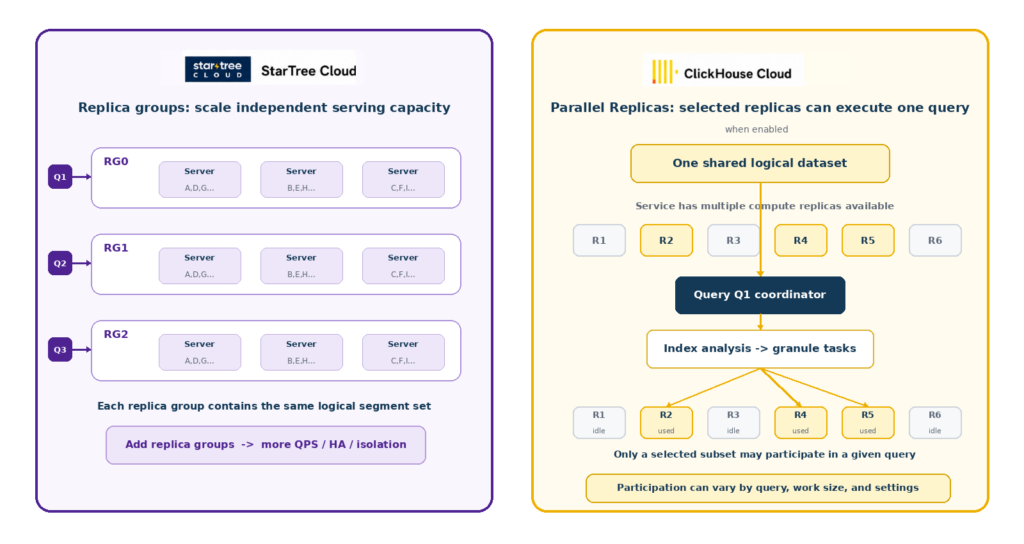
How much parallelism helps, however, depends on how much useful work remains per replica relative to the overhead of coordinating them.
Distributed execution has a coordination cost in either architecture. The distinction is how that distributed work enters the capacity model. Pinot’s leaf execution is distributed across the Servers that already own the relevant segments, so that fanout is part of the normal serving architecture and is accounted for when replica groups are sized. ClickHouse can initially execute a query’s READ work on a single replica, but if the surviving granule set becomes too large for that replica to meet the latency target, Parallel Replicas can turn that same query into a multi-replica scan.
That transition matters because it may not appear in a small POC. As data, query diversity, and working-set size grow, a query that once fit comfortably on one replica can begin recruiting additional workers. Those workers add useful parallelism, but also consume CPU, memory, I/O, and network capacity and introduce coordination work. ClickHouse uses dynamic task assignment and work stealing to reduce the effect of slower participants, while its own Parallel Replicas results show diminishing returns as coordination and network cost grow relative to the useful work left per replica.
Under concurrency, flexibility becomes a capacity question
This changes how the starting replica count should be interpreted. A three-replica ClickHouse service does not necessarily provide three independent units of serving capacity if latency-critical queries routinely recruit multiple replicas. Under sustained concurrency, the shared pool has to be large enough both to accelerate those individual requests and to absorb the other queries arriving at the same time.
Parallel Replicas does not reserve a participating replica exclusively for one query, but the CPU, memory, I/O, and network consumed by that request still reduce the headroom available for other work.
Under sustained QPS, multiple query shapes make overlapping claims on the same replica pool.
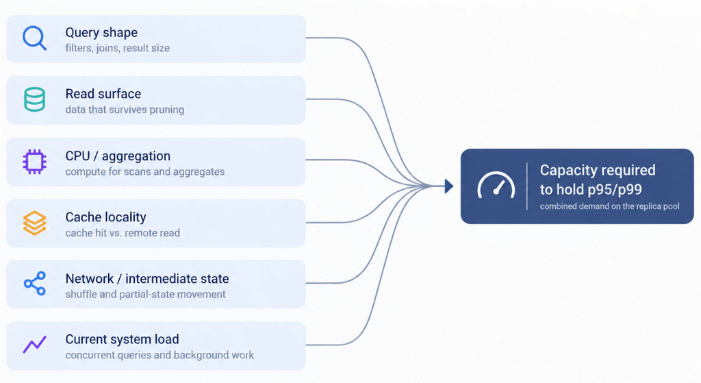
ClickHouse Cloud can add CPU, memory, or replica capacity as demand grows, but elasticity changes when capacity is provisioned, not how much capacity the workload ultimately requires. If latency-critical queries consistently depend on additional workers to preserve the target QPS and p95/p99, those workers become part of the production serving footprint even if they are recruited dynamically.
The ClickHouse Cloud capacity needed to hold that target therefore depends on the query shape, cache state, concurrency, and how many replicas each request uses. Pinot’s leaf data and index ownership remain pre-established, while ClickHouse can vary how much shared compute participates in an individual request.
| Buyer takeaway: Do not compare starting replica counts in isolation. Pinot’s replica-group model uses additional serving copies primarily to add independent throughput, while ClickHouse replicas can also be recruited to accelerate an individual query. If production queries require Parallel Replicas to hold the latency SLO, that shared compute belongs in the production capacity comparison. The useful question is not how many replicas the service starts with, but how much total capacity must remain available to sustain the target QPS and p95/p99. |
Why small tests can hide the production scaling model
A valid POC can test the query without testing the eventual production architecture.
A smaller dataset may contain fewer parts, keep the most useful index state comfortably inside cache and working memory, and make local index analysis cheap enough that distribution provides little benefit.
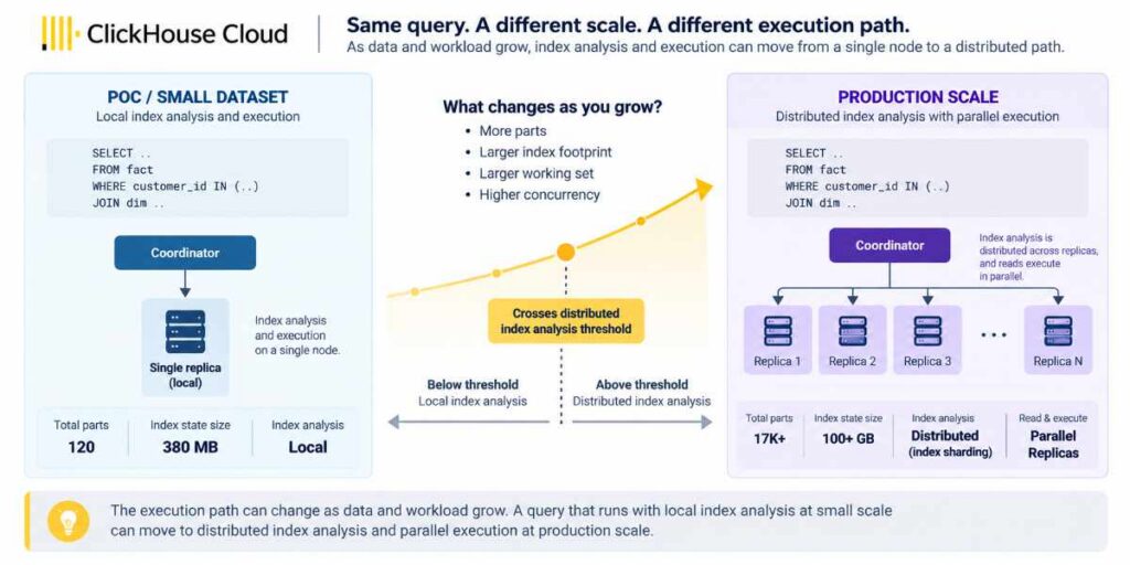
Production can change several things at once: retention and part count, secondary-index footprint, query mix, cache working set, and concurrency. The same query can then require a different execution approach even though the SQL has not changed.
The illustration above shows both ways that transition can happen. If candidate index work grows, FIND can cross from local to Distributed Index Analysis. If PRUNE + FIND still leave enough data that one replica can no longer hold the latency target, READ/execution can cross from single-replica execution to Parallel Replicas.
The Distributed Index Analysis thresholds discussed earlier make the FIND crossover explicit; Parallel Replicas is the analogous READ crossover. A production POC should therefore test not only whether FIND remains local, but whether representative queries can still meet the latency SLO on one replica as the dataset, working set, and query mix grow. If either stage requires distributed workers to hold that SLO, that capacity belongs in the production serving model.
Small POCs are not the only place this happens. Standardized benchmarks fix the dataset, physical design, and query mix in advance.
A standardized benchmark does not reveal the production footprint
ClickBench is valuable because its dataset, queries, configurations, and results are public and reproducible. That still does not make the benchmark representative of production.
ClickBench’s standard rules use one primary index and discourage additional indexes and pre-aggregation, while fine-tuned variants can be published separately for reference. Its 43-query workload is dominated by single-table scans, aggregations, Top-N queries, and broad GROUP BY operations over roughly 100 million rows. That makes it useful for comparing broad analytical execution under a standardized setup. It is a much weaker proxy for production analytical serving, where physical design is not an optional step.
That distinction is visible in the standard configurations. ClickHouse uses a MergeTree primary key of (CounterID, EventDate, UserID, EventTime, WatchID), giving it a sparse primary index and physical ordering. Several later benchmark queries filter on CounterID and EventDate, the leading columns of that key. The standard Pinot configuration defines an empty tableIndexConfig, with no sorted, inverted, range, or Star-Tree indexes. In practice, the benchmark compares ClickHouse with a deliberate physical ordering against Pinot doing much of this workload as a scan-and-aggregate engine. ClickHouse performs very well under that setup, but it is not a production-tuned Pinot configuration.
ClickBench now also publishes a separate tuned Pinot result. That configuration adds only two Star-Tree Indexes and no other workload-specific Pinot indexes. On c6a.4xlarge, reported data size increases by about 1.3%, while the matching SUM(AdvEngineID), COUNT(*), AVG(ResolutionWidth) query drops from 140 ms to 8 ms, a 17.5× improvement. Most other queries change far less because the two Star-Trees cover only a small part of the workload. The result demonstrates the central point of this paper particularly well: a relevant index can dramatically reduce the work for the queries it serves. Under a mixed workload, that can also free capacity for everything else running alongside them.
The tuned run is still narrow. It does not test other normal Pinot design choices such as RAW encoding for appropriate high-cardinality columns, a sorted access path, or filtering indexes. Results from one specific benchmark setup should not be treated as proof that the same behavior will hold in a production-tuned deployment.
That distinction matters because ClickHouse’s May 2026 ClickBench article used the then-published July 2022 Pinot result to draw much broader conclusions about Pinot’s workload fit. It argued that systems completing the benchmark without failures could be deployed against an “arbitrary analytical workload,” while Pinot required workload pre-validation as query diversity increased. The refreshed results materially change that evidence: Pinot 1.5.1 now completes all 43 queries, and the separate Star-Tree-tuned run shows that a relevant index can change query latency by an order of magnitude.
Scale matters too. The standard benchmark uses roughly 100 GB / 100 million rows on a single c6a.4xlarge, and ClickHouse’s compressed representation is about 14 GB on a machine with 32 GiB of RAM. The headline comparison uses hot-cache query timings. That environment says little about what happens when the retained dataset, index footprint, query diversity, cache working set, concurrency, and number of parts grow by orders of magnitude.
A standardized benchmark can tell you how quickly an engine executes the benchmark. It cannot tell you the production footprint required to hold your application’s QPS and p99. The way to close that gap is to test the production SLO directly.
How to measure the production footprint
A production evaluation should start by fixing the application target rather than the cluster size. For example, assume 500 QPS at p99 below 100 ms while representative ingestion is running against a production-like dataset, part or segment count, index footprint, and query mix. Then measure what each architecture requires to sustain it.
Apache Pinot exposes several distinct architectural roles, and those roles respond to different scaling pressures. Servers own segments, indexes, and leaf execution, so their capacity scales primarily with retained data and leaf-level query work. Brokers scale more with query concurrency, result aggregation, query complexity, and MSQE intermediate processing. Minions provide an independent background-processing tier, while Controllers and ZooKeeper/Helix maintain cluster state, placement, and coordination.
That separation lets these parts scale independently. Serving capacity, routing and intermediate processing, background work, and cluster management do not all have to scale together.
ClickHouse Cloud manages more of this supporting infrastructure for the user, including shared storage, caching, metadata and catalog services, load balancing, orchestration, and its control plane, with separate ingestion resources when ClickPipes is used. Fewer visible infrastructure roles do not necessarily mean a smaller serving footprint; the useful comparison is the capacity that changes as the workload grows.
POC metrics that expose the architecture
| Metric | Why it matters |
|---|---|
| p50 / p95 / p99 | Application latency and tail behavior under sustained load |
| Rows / documents processed | Amount of row-level work reaching execution |
| Bytes read / processed | Data volume surviving pruning/indexing |
| Parts / segments considered and processed | How much of the table the engine must consider for the query |
| Granules / documents surviving filters | Effectiveness of pruning and indexing |
| Query mix vs. physical layout | Does the SLO hold across the real application workload, or mainly for queries that align with the table’s physical order? |
| Freshness / ingestion lag under load | Whether new data remains fresh while the system sustains the target query QPS and latency |
| Servers / replicas participating | Per-request distributed fanout |
| Memory and CPU under load | Capacity consumed to hold the SLO |
| Storage / cache behavior under load | Physical cost and sensitivity to locality |
| Total serving footprint | Infrastructure required to sustain target QPS/p99 |
Pinot exposes much of the per-query work directly in the Broker response, including Servers queried and responded, segments queried/processed/matched, documents scanned, and entries scanned during and after filtering. EXPLAIN and MSQE stage statistics provide additional execution detail.
ClickHouse Cloud exposes complementary views through system.query_log, EXPLAIN indexes=1, ProfileEvents, and Parallel Replicas diagnostics. When work executes across replicas, ClickHouse recommends correlating child executions through initial_query_id, because resource usage recorded on the initiating query does not include all remote work.
Repeat the workload while increasing retention, part or segment count, index footprint, query diversity, and concurrency, while keeping the application SLO fixed. The changes required underneath that SLO reveal the production scaling model.
Any capacity that must stay online to preserve the target QPS and p99 is part of the workload’s baseline production footprint. Elasticity only applies to capacity that can be added or removed without breaking that target. This matters when extra compute stops being an occasional accelerator and becomes capacity the workload needs all the time.
That is the thread running through the entire comparison: discovery work determines execution work; execution work determines per-query resource demand; and under sustained serving load, that demand determines the baseline capacity required to hold the SLO.
Conclusion
ClickHouse Cloud and StarTree Cloud can both deliver excellent analytical latency, but they optimize different operating points. A ClickHouse table whose physical design aligns well with an important query family can prune aggressively and execute it very efficiently. ClickHouse Cloud also uses shared storage and elastic compute replicas; with Parallel Replicas enabled, suitable queries can use more nodes at runtime.
StarTree establishes segment ownership, routing, and persistent indexes ahead of the query. Those indexes can reduce selective reads, while Star-Tree Index can combine filtering and pre-aggregation for recurring aggregation-heavy query patterns. MSQE remains available when broader distributed processing is required.
For production serving workloads, latency is therefore only half the result.
The other half is how much physical design, query-time work, and infrastructure are required to keep that latency stable as data, query mix, freshness requirements, and QPS grow.