
The Databricks challenge
At Data + AI Summit in June, Databricks introduced Lakehouse//RT (codenamed Reyden) and made an argument from the main stage that we agree with almost entirely.
It went like this. Low-latency, high-concurrency analytic serving has been dominated by two engines, Apache Pinot and ClickHouse. This is the workload behind customer-facing dashboards, in-app metrics, and increasingly agents. Both engines sit outside the lakehouse, so teams maintain a second copy of their data to get serving performance. Reyden’s promise is that performance without moving data out of your Delta tables.
Two parts of that are exactly right. Databricks named Pinot as one of the reference engines for this workload. And they made the case that serving should be a first-class workload in the modern data platform, not a separate system bolted on downstream.
The part they got wrong is the premise that Pinot requires a second copy. StarTree brought Pinot to the lakehouse, querying external Iceberg and Delta Lake tables in place, and it was generally available before Databricks announced Reyden in private preview.
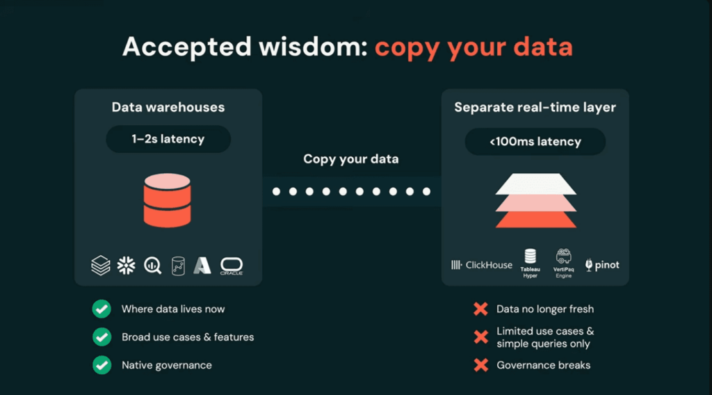
In the subsequent demo, Databricks showed how their new query engine was able to scale to 12,000 queries per second (QPS), on lakehouse data, while Snowflake and Clickhouse fell behind or crashed.
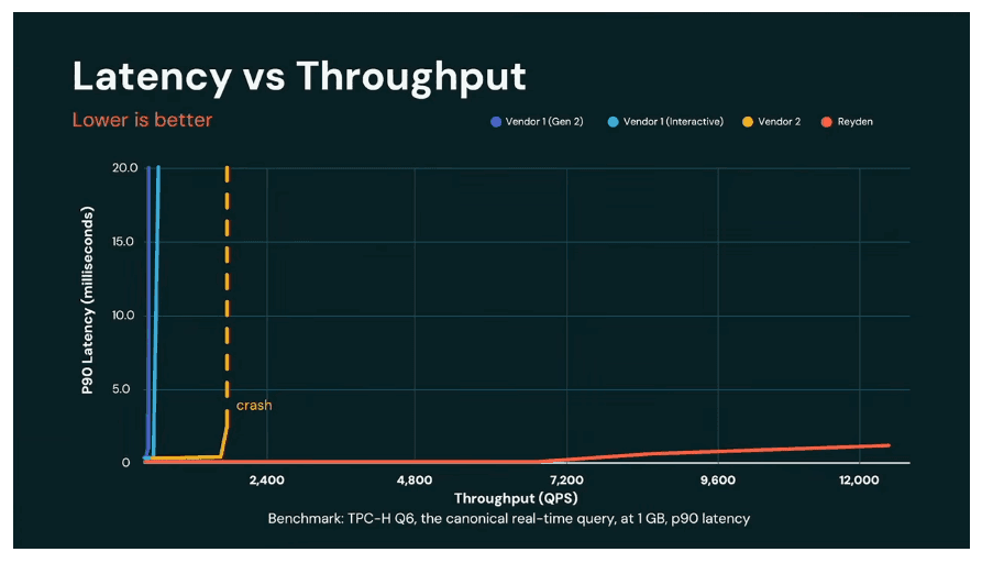
It was unlikely to be the last word on the subject.
Then came the responses
Snowflake and ClickHouse both responded, and the demo opened up a debate about how to benchmark analytics, and what was possible.
The trouble with debating Databricks’ demo is that there isn’t much to debate. They showed more than 12,000 QPS on stage but didn’t publish hardware, query setup, or cache behavior, so no one can reproduce or size the result.
ClickHouse’s response provided more to examine.
They reconstructed what they believed to be the workload—TPC-H Q6 at scale factor 1 with fixed parameters—and published both their methodology and results. A single 30-vCPU ClickHouse Cloud node managed roughly 420 QPS while keeping P90 latency below one second. Adding nodes pushed throughput towards 15,000 QPS.
There was, however, an important difference.
ClickHouse loaded the data into their own native storage format before running the benchmark. That is a reasonable way to demonstrate the serving performance of ClickHouse. However it didn’t quite answer the question Databricks had raised – what happens when the authoritative data stays in the lakehouse?
Snowflake’s response focused on methodology. They argued that Databricks hadn’t configured Snowflake the way it would run in production, and they published TPC-H runs at 100 GB and 1 TB using Interactive Warehouse. They added useful context, but they didn’t include a high-QPS run against externally managed lakehouse data either.
At this point we became curious.
ClickHouse had published enough detail to give us a workload we could reproduce. We decided to run the same basic test with StarTree. And we left the data in lakehouse tables as Databricks had proposed.
Benchmarking StarTree against the Databricks Demo
StarTree is powered by Apache Pinot, which LinkedIn originally built for member-facing analytics.
High query concurrency is not a new problem for Pinot. Production Pinot deployments have long operated at hundreds of thousands of queries per second for workloads in which there is often a person—or an application—waiting for the response.
What has changed is where Pinot can operate.
On StarTree, Pinot can query external Iceberg and Delta Lake tables without first ingesting their rows into Pinot’s storage format. That makes it possible to answer the challenge raised by the Databricks demo.
We started with the publicly identifiable workload ClickHouse identified:
- TPC-H Q6
- TPC-H scale factor 1
- the fixed Q6 parameters published by ClickHouse
- open-loop load generation
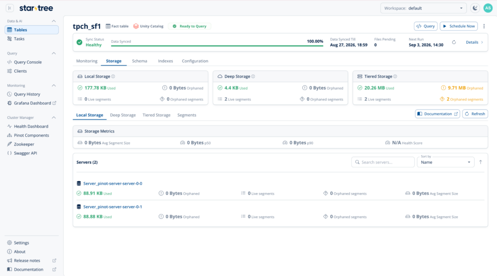
The lineitem table remained as Parquet in S3 and was registered in Unity Catalog as an external table. StarTree queried those files without ingesting the rows into Pinot-managed storage.
StarTree still maintains an acceleration state. Indexes sit alongside the data, and frequently accessed Parquet pages are kept in a bounded local cache. The authoritative table, however, remains in object storage rather than being copied into a duplicate native table.
First: the 12K QPS test
TPC-H SF1 contains 6,001,215 lineitem rows. We used RAW encoding and range indexes on shipdate, discount, and quantity.
The 12-node cluster used:
| Role | Instance | vCPU each | Count |
|---|---|---|---|
| Server | i4g.4xlarge | 16 | 12 |
| Broker | m6g.xlarge | 4 | 12 |
| Controller | m6g.large | 2 | 1 |
That’s 242 vCPUs total.
Traffic was generated with k6 in constant-arrival-rate mode, so the offered workload did not fall simply because the database slowed down. Each load level ran for 45 seconds.
The results:
| Offered QPS | Served QPS | P90 | Errors |
|---|---|---|---|
| 1,000 | 996 | 12.4 ms | 0 |
| 4,000 | 3,995 | 12.6 ms | 0 |
| 8,000 | 7,990 | 13.9 ms | 0 |
| 12,000 | 11,996 | 19.2 ms | 0 |
At 12,000 offered QPS, StarTree served 11,996 QPS at 19.2 ms P90 with zero errors. The same cluster stayed below a one-second P90 through roughly 16,000 QPS.
This test answered the challenge:
StarTree was able to reach the same concurrency class as the Databricks demo without first loading the table into Pinot storage.
Comparing ClickHouse and StarTree results
At this point, it’s worth pausing to compare the results from Clickhouse against StarTree.
The ClickHouse response demonstrated a 20-node configuration that used 600 vCPUs and crossed the one-second P90 threshold at roughly 9,300 QPS.
StarTree’s 12-node configuration only used 240 vCPUs for servers and brokers and was still at 19 ms P90 at 12,000 QPS. Better performance on 40% of the hardware.
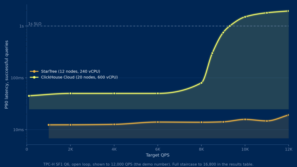
In the original analysis, the ClickHouse curve implied roughly 775 vCPUs to reach 12,000 QPS while remaining below the same one-second P90 threshold.
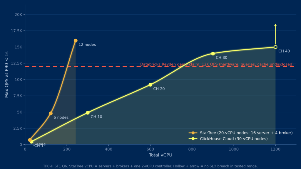
That figure might not be exact. ClickHouse did not publish the underlying raw result table, so the 775-vCPU number is an estimate derived from the chart rather than a measured ClickHouse result.
Even with that caveat, the result caught our attention.
The interesting part was not merely that StarTree appeared to require less compute. It did so while querying an external Parquet table.
That’s not the outcome you might have expected going into the comparison.
Scaling the architecture to 125K QPS (or more)
How well does this scale?
To test this, we kept the storage architecture, data, Q6 workload, and open-loop methodology the same and added compute.
We grew the server tier from 12 to 150 i4g.4xlarge instances, with 120 brokers at the larger scale.
| Servers | Headline QPS | P90 |
|---|---|---|
| 12 | 16,000 | 19ms |
| 120 | 100,000 | 173 ms |
| 150 | 125,000 | 186 ms |
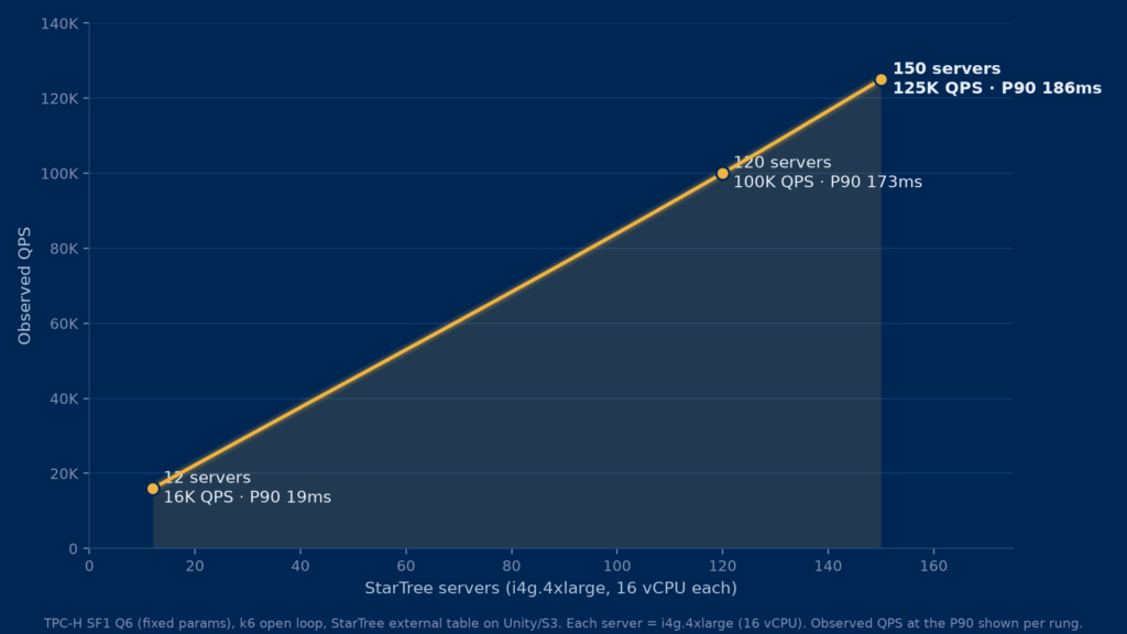
The 150-server configuration reached 125,300 QPS at 186 ms P90.
Looking below the maximum rate:
| Observed QPS | P90 |
|---|---|
| 86,900 | 35 ms |
| 103,300 | 75 ms |
| 125,300 | 186 ms |
At more than 100,000 QPS, P90 was still 75 ms.
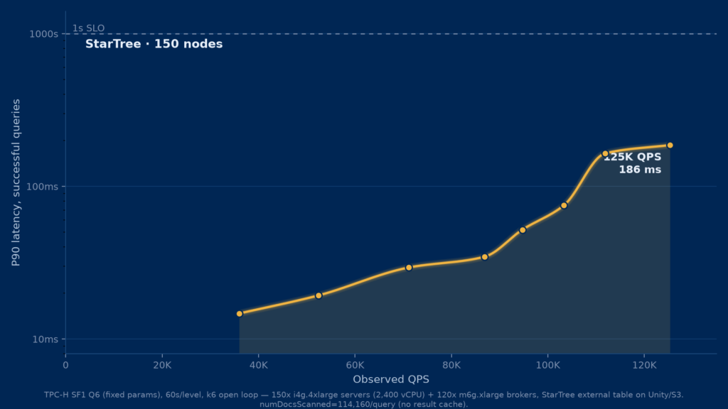
Nothing about the storage path changed to achieve that. Queries were still served against the external Parquet-backed table, with no result cache and no conversion into Native Pinot Segment format.
And to be clear, 125k QPS is not a limit of Pinot’s performance, it was just the limit of our testing budget.
From SF1 to SF100
There is an obvious objection to all of this. Six million lineitem rows is a small dataset, particularly for a system intended to query large lakehouse tables.
So we repeated the Q6 TPC-H experiment at SF100:
| Metric | SF1 | SF100 |
|---|---|---|
lineitem rows | 6,001,215 | 600,037,902 |
| Parquet in S3 | ~200 MB | ~21 GB |
| Compute | 242 vCPU | 242 vCPU |
The SF100 table remained Parquet in S3 and used the same Unity Catalog external-table architecture and 12-node cluster.
At SF100, a straightforward Q6 scan would touch roughly 11.4 million rows per request. Repeating that work thousands of times per second isn’t sensible, so we added a Pinot Star-Tree index on the external table.
We created a new column for the discount price, and pre-aggregated:
SUM(disc_price)
over:
shipdate, discount, quantity
This reduced the documents touched by each query from 114,160 at SF1 to 4,002 at SF100.
| Metric | SF1 | SF100 |
|---|---|---|
| Configuration | RAW + range indexes | RAW + range indexes + Star-Tree |
| Documents/query | 114,160 | 4,002 |
| Offered → served QPS | 12,000 → 11,996 | 12,000 → 11,969 |
| P90 | 19.2 ms | 147.8 ms |
The full SF100 run:
| Offered QPS | Achieved QPS | P90 |
|---|---|---|
| 2,000 | 1,992 | 4.7 ms |
| 4,000 | 3,996 | 20.6 ms |
| 8,000 | 7,985 | 91.0 ms |
| 12,000 | 11,969 | 147.8 ms |
| 14,000 | 13,898 | 221.8 ms |
| 16,000 | 13,922 | 2,739.9 ms |
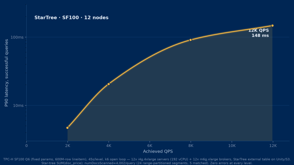
With 100× more rows and no additional compute, StarTree was able to serve almost 12,000 QPS at 147.8 ms P90. At 14,000 offered QPS it remained at 221.8 ms P90; above that, the server tier saturated.
This doesn’t mean that table size has no cost. SF100 uses a different physical optimization because a larger dataset makes repeated scans inefficient.
The more useful point is that the optimization—the Star-Tree index—can be applied directly to the external table. Scaling the workload did not require replacing the open Parquet table with a Pinot-native copy.
What the cache is doing
These are warm-state serving numbers.
Each StarTree server maintains a bounded LRU cache of Parquet pages used by the workload. Pages that are not present locally are fetched from S3. The cache contains the active working set rather than a complete local copy of the table.
So “querying the lakehouse directly” doesn’t mean hitting S3 for every byte on every request. Indexes reduce the amount of data involved, and hot pages move closer to compute.
It also does not mean loading the entire table into another database before it can be served.
What the Databricks, ClickHouse, Snowflake, and StarTree results actually show
Databricks and ClickHouse defined the arena for this study. We met them there.
Databricks validated the need for a high-concurrency query engine that could run on lakehouse storage. But their original benchmarks did not disclose enough configuration detail for an independent reproduction.
Snowflake explained that warehouse sizing and production configuration affects the results, but their response did not demonstrate the same high-QPS workload against externally managed lakehouse data.
ClickHouse published a more reproducible high-QPS test. They were able to match Databricks concurrency by adding compute, but only after they had imported the data into ClickHouse’s native storage format.
Our results prove the point:
Apache Pinot was already designed around high-concurrency analytical serving. With StarTree, that serving model can now be applied to external lakehouse tables.
In our test, StarTree reproduced the general concurrency level of the original Databricks demo without first ingesting the source table into Pinot-managed storage. Against the published ClickHouse workload, it did so with substantially less compute. And when we added servers, the same external-table architecture continued past 125,000 QPS.
Increasing the source table from six million to 600 million rows did not negate that capability either, although doing so sensibly required a different optimization in the form of a Star-Tree index.
This result should not imply that every lakehouse query can become a millisecond query. There are still good reasons to load data into a dedicated serving layer. But it does not need to be a prerequisite for serving high-concurrency analytics.
While limited in scope, this study demonstrates how StarTree can serve application-style analytical workloads from the lakehouse within tens of milliseconds, at high-concurrency, at scale, and without requiring the table to be ingested into a separate serving layer first.
Try it yourself
StarTree customers already run Pinot at hundreds of thousands of queries per second, tens of billions of queries per week, and with SLOs defined against P99 rather than P90.
If your analytical data needs to remain in open lakehouse storage but the applications consuming it need a low-latency, high-concurrency serving layer, talk with us to see how the same approach behaves on your workload.
Bring your catalog and your queries. We can put some numbers against them.