TCO: What Does It Cost to Keep the SLO?

This article is part of a Series comparing ClickHouse Cloud and StarTree. The first article examined query performance and the amount of work each architecture performs per request. Here we follow that question into production economics: what does it cost to keep freshness, QPS, and latency SLOs intact as the workload grows?

Cost-success stories persuade because they put a dollar figure on architecture.

Take these two production snapshots as an example.

ClickHouse Cloud | InMobi	StarTree Cloud | Amberdata
400K+ queries/day 200-600 queries/min P99: >60 sec -> <3 sec $40K/month -> $8K/month	66% infrastructure-cost reduction 350K+ average insert events/sec Nearly 1M peak insert events/sec Sub-second to millisecond query latency
Projects 5x data-volume growth over 2 years Each added node/replica tested at ~30% more traffic	Higher query concurrency while meeting SLAs StarTree Cloud + tiered storage + AZ aware ingestion used to reduce cost

These are not meant as a head-to-head workload comparison. They are snapshots of particular workloads at particular points in time. A buyer still needs to understand what happens when an application retains more history, adds another use case, introduces new query patterns, serves more users, tightens latency objectives, or ingests several times more data ^{[1] [2]}

The InMobi case study makes that growth question unusually explicit. Its current reporting workload runs at roughly 3.3 to 10 QPS, and the team projects data volume to grow 5x over the next two years. Its stress tests showed each additional ClickHouse node or replica handling about 30% more traffic. ClickHouse describes the resulting cost growth as a step function: the bill stays relatively stable until the workload needs another unit of capacity. ^[1]

The full production run rate

At StarTree, we believe that real-time analytics TCO has to include the full cost to serve: storage, ingestion and query compute, background processing, data movement, and operational resources. Our earlier cost work organized the problem around storage, compute, and operational cost, then connected compute efficiency to how much work the system performs for every request. ^[3]

ClickHouse’s recent CostBench work applies a similar full-path lens. It measures the cost of keeping continuously arriving data query-ready together with query-serving cost and runtime. The first end-to-end results used 113.2 billion stock-market rows at a target rate of one million rows per second while analytical queries continued to run. ^{[4] [23]}

That is the right direction. The harder question is how cost evolves once the production workload stops looking like the original benchmark or POC.

Follow the bytes through the full path

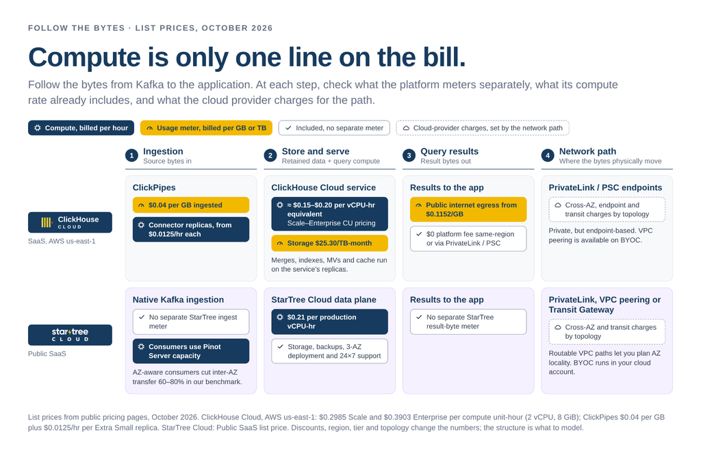
For a streaming ClickHouse Cloud application, the production path can include ClickPipes, database write and merge work, retained storage, indexes and projections, materialized-view maintenance, cache, query compute, result traffic, and cloud-network movement. Several of those dimensions move independently.

Streaming ClickPipes currently starts at $0.0125/hour for one Extra Small replica and also charges $0.04 per GB ingested. Scaling the ClickPipe vertically or horizontally adds connector compute independently of the ClickHouse database service. ^[5]

Superwall makes the volume dimension concrete. ClickPipes moves more than 100 MB/sec of events from WarpStream into ClickHouse Cloud, feeding more than 300 TB of data that is growing by roughly 40 TB each month. At a sustained 100 MB/sec, about 259.2 TB would traverse the ingestion path in a 30-day month. At $0.04/GB, that is about $10,368/month for the volume component alone. This is an illustration of the published meter, not an estimate of Superwall’s private bill. ^{[5] [6]}

Compression downstream does not reduce the bytes that already crossed a volume-metered ingestion boundary. Database compute can still have headroom while ingestion spend rises with source volume.

Query-result traffic scales with QPS

Query-result traffic is approximately QPS x average response size x time. At 100 QPS with an average 25 KB response, a continuously running application returns:

100 QPS x 25 KB x 31,536,000 seconds/year = 78.84 TB/year

If those results leave ClickHouse Cloud over the public internet from AWS us-east-1, where the current published rate is $0.1152/GB, the ClickHouse Cloud data-transfer line is about $9,082/year. At 1,000 QPS with the same response size, the same line becomes about $90,824/year. Response compression, region, application placement, and network topology can materially change the result. ^[7]

ClickHouse Cloud’s platform data-transfer meter is $0 for same-region traffic, and it does not add its own data-transfer fee for PrivateLink or Private Service Connect traffic. That can remove the $0.1152/GB public-internet line. Cloud-provider charges can still remain depending on endpoint processing, cross-AZ paths, transit services, and source-side networking. ^[7]

The platform transfer meter and the underlying cloud-network path therefore need to be modeled separately.

Data movement and network topology

StarTree does not add a separate StarTree ingress or egress usage meter. Underlying cloud-provider network charges can still apply, so the network topology matters. In SaaS, customers can choose PrivateLink when endpoint-based private access is appropriate, or use VPC peering or Transit Gateway when direct VPC-to-VPC routing and greater control over the network path are useful. In BYOC, the data plane runs inside the customer’s cloud account, giving the customer direct control over VPC routing, availability-zone placement, and existing cloud commitments. ^{[8] [12]}

That choice affects more than ingestion. With routable VPC connectivity, application traffic, query results, and streaming data can be designed around the physical region and availability-zone topology rather than simply being sent through a private endpoint. A private path is not necessarily an AZ-local path.

StarTree also uses that locality explicitly for streaming ingestion. AZ-aware Kafka ingestion aligns Pinot consumers with Kafka replicas in the same availability zone where possible, while zone-aware instance assignment preserves placement across the Pinot cluster. In our benchmark, enabling AZ awareness reduced inter-AZ transfer by 60–80%, depending on workload pattern. ClickPipes currently scales Kafka ingestion through one or more consumer replicas in ClickHouse Cloud and does not offer an equivalent AZ-aware Kafka consumer-placement mechanism. ^{[13] [5]}

The same locality question applies on the serving side. StarTree’s routable VPC options let customers consider application placement, query-result traffic, and database placement together, rather than treating private connectivity as the end of the network-design problem.

ClickHouse Cloud SaaS takes an endpoint-based approach to private connectivity through PrivateLink or Private Service Connect. That keeps traffic private, but does not provide the same customer-routable VPC topology for coordinating application, source, and database placement. ClickHouse BYOC is different: because the data plane runs in the customer environment, ClickHouse supports VPC peering there.

So there are three networking questions in a serious TCO model:

What does the platform meter?

What does the cloud provider charge because of where the bytes actually move?

And how much control does the deployment model give you over that physical path?

All three need to be modeled.

Commercial tier and packaging

StarTree Public SaaS currently starts at $0.21 per production vCPU-hour. That price includes the platform, managed service, dedicated infrastructure, compute, storage, autoscaling, backups, security, a standard three-AZ deployment, and 24×7 technical support. We do not add separate StarTree ingestion or storage usage meters. ^[8]

We also do not make a higher compute tier the entry ticket for baseline enterprise capabilities such as SSO. StarTree Cloud includes OIDC-compatible SSO and RBAC as platform security capabilities, and BYOC runs the full data plane inside the customer’s cloud account. ^[12]

ClickHouse Cloud packages some of these capabilities by tier. Its Enterprise tier includes SAML SSO. In AWS US-East, ClickHouse currently lists Scale compute at about $0.30 per compute-unit-hour and Enterprise at about $0.39. One compute unit includes 2 vCPU and 8 GiB of RAM, so on a CPU-only normalization those rates are roughly $0.15 and $0.20 per vCPU-hour. That makes the raw compute rate comparable by CPU count, but not the overall service price: ClickHouse meters storage separately at about $25.30 per TB-month, while ClickPipes ingestion, additional backups, and some data-transfer paths add separate usage dimensions. The current support policy gives committed Enterprise customers a 30-minute Severity-1 initial-response target, compared with one hour for committed Scale and two hours for pay-as-you-go Scale. ^{[9] [10] [11]}

For buyers, the relevant price is the tier that meets their identity, security, support, and compliance requirements, plus the usage meters outside compute

Workload growth crosses capacity boundaries

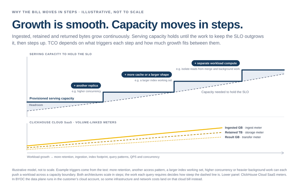
Volume-linked costs tend to rise continuously. More source bytes increase a per-GB ingestion meter. More retained bytes increase storage. More query-result bytes increase network traffic. Serving capacity often behaves differently.

A service can have enough headroom for months. Then more retention, another access pattern, a larger index working set, higher concurrency, or heavier background work pushes the workload across a boundary where another replica, larger compute, more cache, separate merge resources, or additional query workers are needed to preserve the same SLO.

Elastic compute still has to find the data

ClickHouse Cloud’s separation of storage and compute gives replicas flexible access to the same SharedMergeTree data. That elasticity does not remove the work required to determine what a query should read. After partition and part pruning, ClickHouse still analyzes applicable primary and secondary index state to identify surviving granules before data reading begins. ^[14]

As retention grows, the table can accumulate more parts and more index state. As applications add query patterns, additional indexes and access paths can expand the discovery surface further. The final answer may still be five rows while FIND has much more metadata and index state to reason about.

ClickHouse has introduced Distributed Index Analysis, currently in private preview for SharedMergeTree, because this work can become large enough to distribute. On its published 50-billion-row test with about 17,000 parts and six million marks, a Bloom-filter lookup spent 8.5 seconds in index analysis without distribution. With 10 replicas participating, that fell to 1.1 seconds; with 20 replicas it fell to 0.65 seconds. ^[14]

Storage can scale independently from compute, while the cost of finding the relevant data still has to be paid somewhere.

More replicas can make that analysis faster and spread index memory across the fleet. Economically, the point is that preserving the same p99 can require more participating compute as the discovery problem grows. ^[14]

Production scaling in practice: Exabeam

Exabeam runs ClickHouse Cloud across 10 global regions, reaches about 1.2 million events/sec per region, processes more than 80 billion events/day, and has stored more than one trillion events. At that scale it separated write, merge, and read workloads onto dedicated compute so heavy reads would not interfere with ingestion and merges. ^[15]

The team also encountered part growth from backdated events landing across historical partitions. It split ingestion into real-time and backlog paths so older events could be batched more efficiently, reducing part count and operational overhead. Some N-gram indexes were effective for specialized searches but required enough hardware that Exabeam moved the less-than-1% regex workload to a leaner indexing approach. ^[15]

Exabeam’s experience is also a warning against extrapolating a small POC by row count alone. Parts, index footprint, query diversity, background work, and isolation requirements can all change the capacity needed to preserve the same application behavior.

Doesn’t the same growth apply to StarTree?

Yes. 

StarTree is not exempt from workload growth. More retained data increases the storage footprint, while higher traffic, larger index and mutable-state footprints, and background processing can require additional compute and memory. Indexes consume storage and build resources. Materialized views require storage and refresh work. Upserts maintain state. Background tasks need capacity.

Both systems eventually scale. The economic question is how much workload growth the existing serving footprint can absorb before the next capacity step is required.

StarTree provides several ways to move bounded work ahead of the repeated request path, then choose the mechanism that fits the query pattern.

• Resolve mutable state early. Full and partial upserts establish latest-state visibility during ingestion, so later queries operate against the valid record set instead of repeatedly resolving row versions.
• Place and route early. Segment ownership, persistent index placement, and Broker routing state are established before the query arrives.
• Eliminate records early. Inverted, range, JSON, sparse, text, and other indexes narrow the candidate records before projected values enter general execution.
• Reuse recurring work. The Star-Tree index can pre-aggregate a family of recurring analytical patterns, while materialized views are useful when a stable aggregation or join is better persisted as derived state.
• Distribute broad work when needed. MSQE provides broader distributed execution without changing the basic ownership and leaf-data model.

These mechanisms carry costs of their own. The value comes from how much repeated CPU, I/O, memory, network movement, and runtime aggregation they remove as the application grows. [16] [17]

ClickHouse has its own ways to move work earlier through materialized views, projections, and physical layout. For either system, the useful test is:

How much work can the system do once, how many future queries can reuse it, and how much serving compute does that save?

Work reduction delays the next capacity step

How much work can the system do once, how many future queries can reuse it, and how much serving compute does that save?

That work-reduction model also shows up in production. A major global bank moved its fraud-detection analytics from Bigtable to StarTree and reduced p99 query latency from 300 ms to 50 ms, with p50 as low as 7 ms, while supporting bursts of up to 1,200 QPS and more than 300,000 queries per day. The case study credits an inverted index with reducing query work while also improving TCO. ^[24]

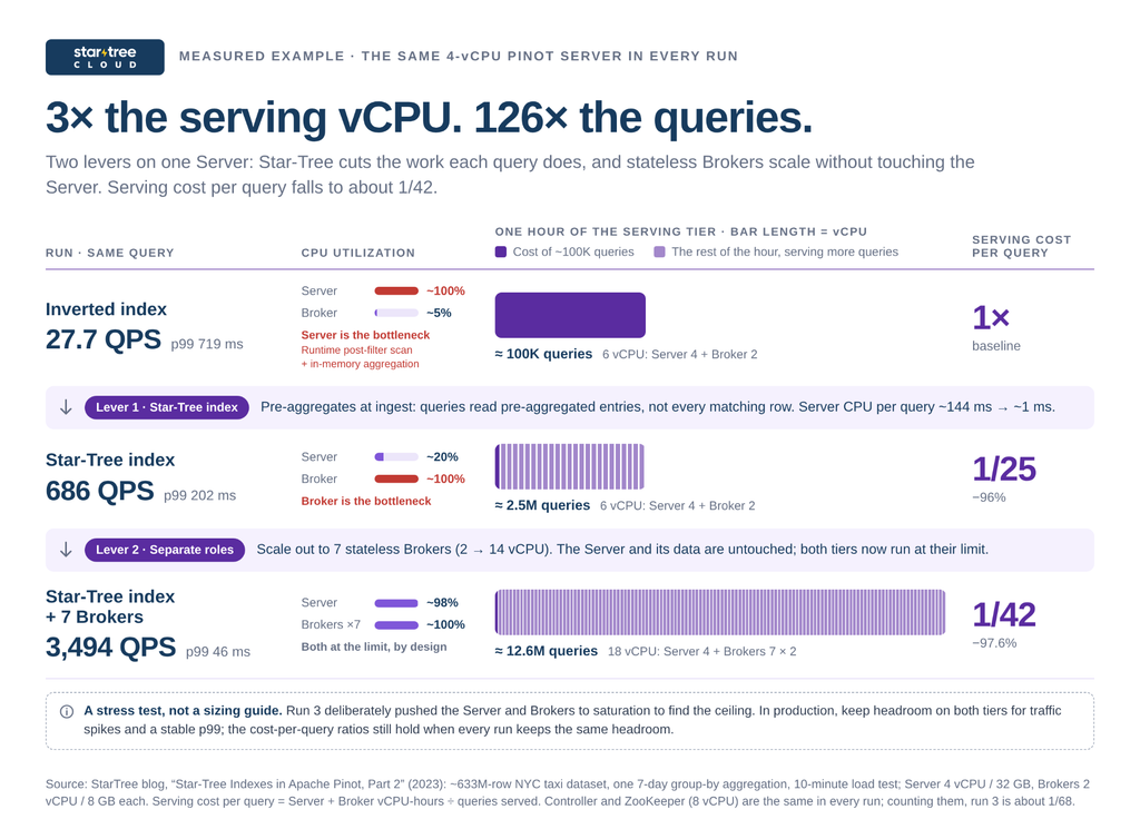
We can also see the TCO effect directly in our Star-Tree index concurrency test. With an inverted-index execution path, a 4-vCPU Pinot Server saturated at about 27.7 QPS with p99 around 719 ms. After adding a Star-Tree index, the same Server handled about 686 QPS at 202 ms p99 while Server CPU was only about 20%. The bottleneck had moved to the Broker. ^[18]

We then scaled the Brokers from one node to seven (2 vCPU each), leaving the same Server in place. Counting those Brokers, the serving tier grew from 6 to 18 vCPU, about 3x, while throughput grew 126x, so serving cost per query fell to roughly 1/42.

The Server did not become 126 times larger. The amount of work each request asked it to perform dropped dramatically.

The companion query test shows why. The inverted index had already eliminated the filtering scan, yet roughly 146 million matching documents still had to be read and aggregated at query time. The Star-Tree index reduced that to 409 documents and 2,045 entries, taking latency from 1,513 ms to 4 ms. ^[19]

At low concurrency, removing that work mostly improves latency. As concurrency rises, every avoided read, decode, aggregation, and intermediate operation becomes capacity available for another request. That changes when another Server is required.

Retention can use different serving tiers

ClickHouse Cloud already separates compute from storage. Native SharedMergeTree keeps authoritative native-table data in shared object storage while compute and cache sit in front of it. That makes retained storage economical and allows compute to scale independently.

For demanding sub-second, high-concurrency serving over lake data, ClickHouse’s own guidance still points back to loading the data into MergeTree so native indexes, compression, and data-skipping optimizations can be applied. Once copied into MergeTree, that retained data belongs to the same SharedMergeTree serving model. As the native dataset grows, more read services, more cache, Parallel Replicas, or distributed index analysis can add resources around the growing table to preserve latency. ^[20]

StarTree lets the application choose among three serving/storage modes as retention grows:

Native Pinot	Tiered Storage	External Tables
Tightest local serving path Native segment values + indexes	Colder segments on remote object storage Pinot segment/index model preserved	Source data stays in Iceberg / Parquet Routing, indexes and caches accelerate serving

Tiered Storage can move colder segment data to object storage while preserving Pinot’s segment and index model. External Tables go further: source data remains in Iceberg or Parquet (no copy or conversion to Pinot Native format) while routing, persistent indexes, and cache state reduce the remote work required by the application. ^{[21] [22]}

How much state needs to remain close to compute to preserve the SLO?

That question can have a very different answer from the total size of retained history. In our External Tables benchmark, roughly 12 billion rows and 1 TB of Iceberg data remained in the lake while about 300 GB of Pinot indexes were configured across four Servers. Selective workloads sustained sub-second latency and hundreds of QPS, including 500+ QPS for some query patterns, without copying the raw table into native Pinot storage. ^[22]

Growth therefore does not automatically force all historical data onto the same serving tier in StarTree Cloud. The application can keep the storage economics aligned with how that history is actually accessed.

Confirm during pricing

Before comparing projected bills, confirm:

• Which commercial tier do our SSO, security, compliance, and support requirements require
• Which costs are included in the base compute price, and which are separately metered?
• Is streaming ingestion charged by source volume, connector compute, or both?
• Which network and deployment options are available: private endpoint, VPC peering, Transit Gateway, or deployment inside our cloud account?
• Can the deployment preserve availability-zone locality for ingestion and application traffic, and who pays any remaining cross-AZ or endpoint-processing charges?
• How is query-result traffic charged?
• What serving capacity must remain provisioned to preserve the required freshness, QPS, and p99 as the workload grows?

A POC is one point on the curve

A conventional POC fixes a dataset, runs representative queries, finds a configuration that meets the latency target, and compares the resulting bill. That establishes one point on the capacity curve.

The useful question is how much additional data, QPS, and query diversity the current footprint can absorb while the application SLO stays fixed.

A production evaluation should test the curve itself. Start with a fixed application contract, for example 500 QPS, p99 below 100 ms, the required freshness window, and production-like ingestion running continuously. Then grow the workload while holding those objectives fixed.

• Increase retention and incoming volume.
• Increase concurrency and average result payload.
• Add another application and new query patterns.
• Add the indexes, projections, Star-Tree indexes, or materialized views the workload genuinely needs.
• Introduce the joins and aggregations production will actually execute.
• Keep background maintenance, ingestion, and failure-domain requirements active during the test.

Track the bill and the work underneath it: ingested GB, retained storage, query-result GB, parts or segments considered, granules or documents surviving filters, rows and bytes processed, index-analysis work, CPU and memory, remote I/O, Servers or replicas participating, background merge or refresh work, and total serving footprint required to hold the SLO.

Then record the transitions. Did the service need another database replica? Did FIND become distributed? Did read and merge workloads need separate compute? Did the ingestion connector need more replicas? Did another cache tier become necessary? Did a Star-Tree index or materialized view let the existing Server footprint keep absorbing growth?

Don’t price Day 1. Hold the freshness, QPS, and p99 targets fixed, then grow retention, query patterns, concurrency, and ingestion. Measure when each architecture needs the next unit of capacity and what new meters appear along the way.

Conclusion

ClickHouse Cloud and StarTree Cloud can both deliver strong cost outcomes when they replace an analytical architecture poorly matched to the workload. What matters comes after that first win: what happens to the run rate as retention, ingestion, query diversity, and concurrency grow?

Both platforms can add capacity. ClickHouse Cloud brings elastic compute, independently scaled ingestion, materialized views, projections, and distributed execution. StarTree’s levers sit earlier in the request path: ownership and routing set before the query arrives, indexes and pre-aggregation where they pay off, and storage tiers that match how history is accessed.

The difference is how far the current footprint stretches. In our test, the same 4-vCPU Server ultimately went from about 28 to 3,494 QPS: first by reducing per-query work with a Star-Tree index, then by adding stateless Brokers after the bottleneck moved upstream. The Server itself never got bigger. Each query simply asked it to do less. 

That is what to measure in your own evaluation: not what Day 1 costs, but how much growth each architecture absorbs before it needs the next unit of capacity, and which meters start running along the way.

Sources and further reading

Product behavior and pricing evolve quickly. The source notes below link directly to the public references used for version-sensitive claims in this article.