
AI agents are becoming production software. One agent request can fan out into dozens of model calls, tool calls and retries, each a row of telemetry. At a million requests a day that’s tens of millions of rows. Every model call, tool invocation, retrieval operation and hand-off leaves behind a trace. As agents become more widely deployed, these traces are quickly turning into one of the largest and most valuable telemetry streams a company produces.
Today, platforms such as Langfuse provide the infrastructure to capture, process and analyze these traces. In its v3 architecture, Langfuse uses a combination of object storage, Redis-backed queues and ClickHouse as its analytical database. This is a practical architecture, and it works well for getting started. But as trace volume and query traffic grow, some of the underlying design choices become harder to manage.
The challenge is that agent trace analytics has to support several different requirements at once. Engineers need to retrieve individual traces quickly, while product and engineering teams need to run analytical queries across millions or billions of observations. The system also needs to handle high-cardinality identifiers, retain large volumes of historical data, and support replay when processing or enrichment logic changes.
ClickHouse is a powerful analytical database, but using it for a single OLAP store as both the trace-serving layer and the long-term home for all trace data creates architectural trade-offs. There is an opportunity to approach the problem differently by separating event processing, durable storage and serving.
In this post, I’ll walk through an architecture built around four components: Apache Kafka for event transport, Apache Flink for stateful processing, Apache Iceberg for durable storage, and StarTree, built on Apache Pinot, for real-time serving.
The goal isn’t to introduce another agent observability platform. It’s to look at how the data infrastructure behind agent traces can be designed to scale.
What is agent trace analytics?
A single request to an agent can trigger dozens of operations: an LLM generation, a tool call, a retrieval lookup, a sub-agent hand-off or a retry. Each operation contributes to the overall execution of the request.
The data model emerging across the industry, and increasingly reflected in the OpenTelemetry GenAI semantic conventions, has a few core entities:
- Trace: A logical request or task from beginning to end. It carries context such as the user, session, project and environment.
- Observation (span): An individual operation within a trace, such as an LLM generation, tool call or retrieval. Observations can be nested, so a trace is a tree rather than a flat list.
- Session: A collection of traces associated with the same conversation or workflow.
- Score: An evaluation attached to a trace or observation. It could come from a human reviewer, a deterministic rule or an LLM acting as a judge.
These entities support two distinct query patterns.
The first is retrieving an individual trace. An engineer investigating a failed request needs to fetch all observations associated with a trace ID, in the right order, along with their inputs, outputs, timing and status. This is a selective lookup over a small number of rows.
The second is analyzing traces in aggregate. Teams want to understand cost per customer, token usage by model, p95 latency by tool, quality scores by prompt version, or regressions following a release. These queries scan and aggregate large volumes of data.
Both patterns matter. Agent execution is non-deterministic, so reproducing a failure by running the same request again may not produce the same result. The trace is often the only record of what happened. At the same time, every model and tool invocation has a cost, making near-real-time visibility into usage important.
The architecture needs to make individual traces easy to retrieve while also making the full history useful for analytics.
How trace analytics systems are typically built
A number of open-source and commercial platforms have emerged in this category, including Langfuse, LangSmith, Arize Phoenix and Braintrust. Their implementations differ, but a common architecture is to accept events through an ingestion API, process them asynchronously, and write the resulting records to an analytical database.
Langfuse is a useful example because its v3 architecture is documented publicly. At a high level, the system works as follows:
- An ingestion API authenticates requests and validates the event payload.
- Raw events are written to blob storage, while a reference to each event is placed on a Redis-backed job queue.
- Workers read the events, reconcile updates to the same trace or observation, calculate token usage and cost, and produce complete records.
- The resulting records are written to a columnar OLAP database, which serves both the trace viewer and analytical dashboards.
- A relational database stores users, projects, API keys and prompt versions.
This is a sensible design, particularly for teams that aren’t already operating streaming infrastructure. But there are a few architectural considerations that become more important as the workload grows.
Point lookups and analytical queries have different access patterns. Retrieving a trace means filtering on a trace ID and returning a relatively small number of observations. Analytical queries, on the other hand, scan much larger portions of the dataset and aggregate across dimensions. A serving engine needs to support both efficiently. The choice of partitioning, indexes and query execution strategy matters.
Trace data grows quickly. Prompts, completions and other payloads can be large, and retaining months or years of history in a serving database can become expensive. Separating long-term storage from the serving layer makes retention and cost management easier.
High cardinality is intrinsic to the data model. Trace IDs, observation IDs, session IDs and user IDs are naturally high-cardinality fields. They are also the fields that applications frequently filter on. The serving layer needs to be designed around these access patterns rather than treating high cardinality as an exceptional case.
The data has value outside the trace viewer. Finance teams may want to join usage with billing data. Data science teams may want to analyze traces alongside training data. Product teams may want to build customer-facing usage analytics. Keeping an open, durable copy of the data makes these use cases easier to support without putting every query on the serving database.
These requirements suggest separating event processing, durable storage and serving, while keeping the same enriched records available to each layer.
A streaming-first architecture: Kafka, Flink, Iceberg and StarTree
The architecture uses Kafka as the event log, Flink to reconcile and enrich events, Iceberg as the durable historical store, and StarTree for serving both trace lookups and analytical queries.
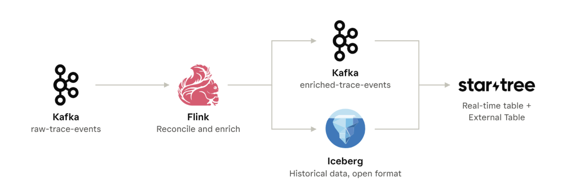
The important design choice is that Flink processes each observation once. After reconciliation and enrichment, the same complete records are written to the serving and storage layers.
How an event moves through the system
1. Ingest
SDKs, or an OpenTelemetry Collector when native OTLP support is required, send events to a thin ingestion API.
The API handles authentication and payload validation. Large prompt and completion bodies, images and files are written directly to object storage. The event carries a reference URI rather than embedding the full payload.
This keeps large objects out of the event stream and follows the external-reference pattern used by the OpenTelemetry GenAI conventions.
2. Log
Events are written to a Kafka topic named raw-trace-events.
The topic is partitioned by trace_id. This ensures that events belonging to the same trace are consumed in order by the same Flink task, making per-trace state management straightforward.
Kafka also provides a durable event log. Consumers can replay events from an earlier offset, which becomes important when processing logic changes.
3. Enrich
A Flink job consumes raw-trace-events and maintains state for each trace.
Events for an observation may arrive as separate create and update messages. Flink reconciles these into a complete record, handles late and out-of-order events, fills in missing token counts, and calculates estimated cost using the applicable model pricing.
It also flattens the trace tree into rows. Each observation retains its trace_id and parent_observation_id, along with trace-level context such as project, user and session.
Once an observation is complete, Flink emits a record with a stable ID.
4. Serve
The enriched records are written to a second Kafka topic, enriched-trace-events.
StarTree ingests this topic into a real-time Apache Pinot table. New observations become queryable within seconds, making the data available for trace retrieval and analytical queries while the agent workload is still active.
5. Persist
The same enriched stream is written to Iceberg tables for observations, traces and scores.
Iceberg provides the durable, open-format copy of the data. It supports long-term retention and allows other engines and teams to query the history without depending on the serving cluster.
6. Query historical data
Recent observations are served from the real-time Pinot table. Historical observations remain in Iceberg and are queried in place through a StarTree External Table.
The real-time and external tables are exposed as a hybrid table. StarTree’s broker combines the two sources under one table name, so applications can query recent and historical observations without having to determine where an individual record resides.
7. Evaluate
Evaluators can consume enriched-trace-events independently. Rule-based evaluators and LLM-as-judge workflows can write scores back through the same pipeline.
This keeps evaluation processing decoupled from ingestion and serving. Adding another consumer does not require changing the upstream event flow.
Responsibility by component
| Component | Responsibility |
|---|---|
| Ingestion API / OpenTelemetry Collector | Authentication, payload validation and offloading large objects |
| Kafka | Durable, ordered and replayable event log |
| Flink | Stateful reconciliation, enrichment and flattening |
| Iceberg | Long-term storage, historical queries, backfills and joins with other datasets |
| StarTree (Apache Pinot) | Low-latency serving for trace lookups and analytical queries |
| Relational database and cache | Users, projects, API keys and prompt definitions |
Why Pinot and StarTree for serving? Three properties fit this workload:
Built for sub-second answers at high QPS. Pinot was designed for user-facing analytics, where many concurrent queries each need a fast answer, so it can back customer-facing trace views and agents querying at run time.
Flexible indexing for multi-dimensional analytics. Sorted, inverted, range, bloom-filter and star-tree indexes are chosen per column, so the same table serves single-trace lookups and slice-and-dice rollups across project, model, tool and time.
First-class Iceberg support. StarTree queries Iceberg tables in place through External Tables, so recent and historical traces sit behind one query surface without copying the lake into the serving layer.
The control plane remains in a relational database. Users, API keys and prompt definitions are transactional entities that need strong consistency. There is no reason to move them into the streaming architecture.
Putting the architecture together
Let’s look at a concrete implementation.
The infrastructure consists of Kafka, a Flink cluster, an Iceberg REST catalog backed by object storage, and StarTree for serving.
The event model
The Kafka message represents one observation, not an entire trace. A trace is the collection of observations sharing the same trace_id.
For example:
{
  "trace_id": "9f1e2a-...",
  "observation_id": "obs-0041",
  "parent_observation_id": "obs-0040",
  "type": "GENERATION",
  "project_id": "proj_7a2",
  "session_id": "sess-cc12",
  "user_id": "user_881",
  "start_time": "2026-11-13T18:22:04.112Z",
  "end_time": "2026-11-13T18:22:05.887Z",
  "model": "claude-sonnet-5",
  "input_tokens": 842,
  "output_tokens": 311,
  "input_ref": "s3://raw-payloads/proj_7a2/obs-0041/input.json",
  "output_ref": "s3://raw-payloads/proj_7a2/obs-0041/output.json",
  "status": "SUCCESS"
}
Code language: JSON / JSON with Comments (json)
The input_ref and output_ref fields point to the full input and output payloads in object storage. The event itself contains the metadata required for filtering and aggregation.
This distinction is useful. Most analytical queries do not need to read the full prompt or completion. Keeping large payloads outside the analytical row reduces the amount of data that needs to move through Kafka and the serving engine.
Enrichment with Flink SQL
A note on reconciliation. SDKs send each step in pieces: a create event when it starts and updates as it runs and finishes. Every trace platform has to merge those pieces into one complete record before serving it. Langfuse does this in its worker service; here, Flink does it with a keyed state before records reach Kafka and Iceberg. Because this is standard plumbing rather than something new in this design, the recipe below leaves it out and shows only the enrichment.
Flink consumes the raw events and writes the enriched output to two destinations: Kafka for serving and Iceberg for durable storage.
The following example shows the structure of the pipeline. The source is a Kafka table:
CREATE TABLE raw_trace_events (
    trace_id STRING,
    observation_id STRING,
    parent_observation_id STRING,
    type STRING,
    project_id STRING,
    session_id STRING,
    user_id STRING,
    start_time TIMESTAMP(3),
    end_time TIMESTAMP(3),
    model STRING,
    input_tokens INT,
    output_tokens INT,
    input_ref STRING,
    output_ref STRING,
    status STRING,
    WATERMARK FOR end_time AS end_time - INTERVAL '5' SECOND
) WITH (
    'connector' = 'kafka',
    'topic' = 'raw-trace-events',
    'properties.bootstrap.servers' = 'kafka:9092',
    'format' = 'json',
    'scan.startup.mode' = 'earliest-offset'
);Code language: PHP (php)
The enriched output topic includes additional fields such as duration, total tokens and estimated cost:
CREATE TABLE enriched_trace_events (
    trace_id STRING,
    observation_id STRING,
    parent_observation_id STRING,
    type STRING,
    project_id STRING,
    session_id STRING,
    user_id STRING,
    start_time TIMESTAMP(3),
    end_time TIMESTAMP(3),
    duration_ms BIGINT,
    model STRING,
    input_tokens INT,
    output_tokens INT,
    total_tokens INT,
    estimated_cost_usd DOUBLE,
    input_ref STRING,
    output_ref STRING,
    status STRING
) WITH (
    'connector' = 'kafka',
    'topic' = 'enriched-trace-events',
    'properties.bootstrap.servers' = 'kafka:9092',
    'format' = 'json'
);
Code language: SQL (Structured Query Language) (sql)
The iceberg catalog can be configured using an Iceberg REST catalog:
CREATE CATALOG iceberg_catalog WITH (
    'type' = 'iceberg',
    'catalog-type' = 'rest',
    'uri' = 'http://iceberg-rest:8181',
    'warehouse' = 's3://warehouse/',
    's3.endpoint' = 'http://minio:9000'
);Code language: SQL (Structured Query Language) (sql)
The observations table stores the enriched records:
CREATE TABLE iceberg_catalog.agent_traces.observations (
    trace_id STRING,
    observation_id STRING,
    parent_observation_id STRING,
    type STRING,
    project_id STRING,
    session_id STRING,
    user_id STRING,
    start_time TIMESTAMP(3),
    end_time TIMESTAMP(3),
    duration_ms BIGINT,
    model STRING,
    input_tokens INT,
    output_tokens INT,
    total_tokens INT,
    estimated_cost_usd DOUBLE,
    input_ref STRING,
    output_ref STRING,
    status STRING
) PARTITIONED BY (project_id, days(start_time));Code language: SQL (Structured Query Language) (sql)
The enrichment logic calculates duration and cost using the pricing table applicable at the observation’s event time:
CREATE VIEW enriched AS
SELECT
    e.trace_id,
    e.observation_id,
    e.parent_observation_id,
    e.type,
    e.project_id,
    e.session_id,
    e.user_id,
    e.start_time,
    e.end_time,
    TIMESTAMPDIFF(MILLISECOND, e.start_time, e.end_time) AS duration_ms,
    e.model,
    e.input_tokens,
    e.output_tokens,
    e.input_tokens + e.output_tokens AS total_tokens,
    (
        e.input_tokens * p.input_price_per_1k +
        e.output_tokens * p.output_price_per_1k
    ) / 1000.0 AS estimated_cost_usd,
    e.input_ref,
    e.output_ref,
    e.status
FROM raw_trace_events e
LEFT JOIN model_pricing
    FOR SYSTEM_TIME AS OF e.start_time AS p
    ON e.model = p.model_name;Code language: SQL (Structured Query Language) (sql)
A Flink statement set writes the same enriched records to both destinations:
EXECUTE STATEMENT SET
BEGIN
    INSERT INTO enriched_trace_events
    SELECT * FROM enriched;

    INSERT INTO iceberg_catalog.agent_traces.observations
    SELECT * FROM enriched;
END;Code language: SQL (Structured Query Language) (sql)
In a production implementation, the state and checkpoint configuration, event-time handling and sink delivery guarantees need to be configured to match the required correctness semantics. The important architectural point is that reconciliation and enrichment happen before the data reaches either serving or historical storage.
Serving with StarTree
The serving layer has two parts: a real-time Pinot table and an External Table over Iceberg.
The real-time table consumes the enriched Kafka topic:
{
  "tableName": "agent_observations",
  "tableType": "REALTIME",
  "segmentsConfig": {
    "timeColumnName": "start_time",
    "timeType": "MILLISECONDS"
  },
  "streamConfigs": {
    "streamType": "kafka",
    "stream.kafka.topic.name": "enriched-trace-events",
    "stream.kafka.broker.list": "kafka:9092",
    "stream.kafka.consumer.type": "lowLevel"
  },
  "tableIndexConfig": {
    "invertedIndexColumns": [
      "project_id",
      "model",
      "trace_id"
    ],
    "sortedColumn": [
      "start_time"
    ]
  }
}Code language: JSON / JSON with Comments (json)
The historical table points to the Iceberg REST catalog:
{
  "tableName": "agent_observations",
  "externalCatalog": {
    "type": "iceberg-rest",
    "uri": "http://iceberg-rest:8181",
    "warehouse": "s3://warehouse/",
    "namespace": "agent_traces",
    "table": "observations"
  },
  "tableIndexConfig": {
    "invertedIndexColumns": [
      "project_id",
      "model",
      "trace_id"
    ],
    "sortedColumn": [
      "start_time"
    ],
    "rangeIndexColumns": [
      "duration_ms",
      "estimated_cost_usd"
    ]
  }
}Code language: JSON / JSON with Comments (json)
The real-time table provides low-latency access to newly ingested observations. The External Table queries the historical Parquet data in place, by leveraging Pinot indexes without having to copy the entire historical dataset into the serving store.
The time boundary is an important part of this setup. It represents the point up to which the historical source is authoritative. The broker uses it to split a query into two time ranges: records at or before the boundary are read from the Iceberg External Table, and records after it are read from the real-time table. The two result sets are merged before being returned. The result is one query interface over recent and historical observations. Applications do not need to manage the two sources themselves.
StarTree has also demonstrated that this serving model can scale to high concurrency while keeping the authoritative data in open lakehouse storage. In a published TPC-H benchmark, StarTree queried an external Parquet table in S3 without ingesting the data into Pinot-managed storage. On a 6-million-row dataset, a 12-node cluster served nearly 12,000 QPS at 19.2 ms P90 latency. Scaling the same architecture to 150 servers pushed throughput to more than 125,000 QPS at 186 ms P90. The team also tested a 600-million-row dataset (approximately 21 GB) on the original 242-vCPU cluster, achieving nearly 12,000 QPS at 147.8 ms P90 with a Star-Tree index on the external table. These are TPC-H benchmark results, not agent-trace measurements, but they demonstrate that historical data can remain in open table formats while still supporting high-concurrency analytical queries. Source: StarTree’s open-tables benchmark.
The hybrid table presents both sources under the same table name. Applications can issue a query without having to route it to a real-time or historical table themselves.
Querying traces and analyzing behavior
The same table supports both individual trace retrieval and aggregate analytics.
To retrieve one trace:
SELECT
    observation_id,
    parent_observation_id,
    type,
    model,
    duration_ms,
    estimated_cost_usd,
    status
FROM agent_observations
WHERE trace_id = '9f1e2a-...'
ORDER BY start_time ASC;Code language: JavaScript (javascript)
This query filters on a single trace ID and returns the observations that make up the trace. The parent_observation_id field preserves the relationships needed to reconstruct the trace tree.
An aggregate query can analyze latency and cost by model:
SELECT
    model,
    PERCENTILE(duration_ms, 95) AS p95_latency_ms,
    SUM(estimated_cost_usd) AS total_cost_usd,
    COUNT(*) AS call_count
FROM agent_observations
WHERE start_time > ago('PT24H')
GROUP BY model
ORDER BY total_cost_usd DESC;Code language: SQL (Structured Query Language) (sql)
Both queries use the same serving table. One retrieves a small set of rows using a trace ID; the other scans a larger time range and aggregates by model.
This is an important property of the architecture. Trace retrieval and aggregate analytics do not have to be separate applications backed by separate serving systems. With the right data layout and indexing, they can run on the same analytical platform.
Design considerations
There are a few choices that have a significant impact on how well this architecture performs.
1. Design the serving layer for both query patterns
Trace analytics is a good example of a workload that combines selective lookups with large analytical queries.
Pinot was designed for low-latency, high-concurrency analytical workloads. In this architecture, inverted indexes on fields such as trace_id, project_id and model help narrow the set of rows a query needs to examine. Sorted columns and range indexes can further optimize time- and value-based filters. Star-tree indexes can pre-aggregate frequently used dimensions for dashboards, such as project, model, tool and time.
The exact index configuration should follow the queries the application actually runs. A trace viewer may primarily filter on trace_id, while a cost dashboard may group by project, model or tool. Both patterns can be supported by the same table, with indexes selected for the access patterns that matter.
2. Use trace ID as a partitioning key
Trace ID is one of the most important fields in the data model. It is high-cardinality by nature, but that is also what makes it useful for selective lookups.
Partitioning segments by trace ID allows Pinot to prune segments that cannot contain the requested trace. The inverted index then narrows the search within the relevant segments.
This is different from treating high cardinality as a storage problem to avoid. For trace retrieval, distinct IDs are valuable because they make lookups selective. The important part is to choose a partitioning strategy that aligns with the query workload and to manage segment sizing and distribution appropriately.
The same key can be used across Kafka, Flink and Pinot. Kafka keeps a trace’s events together, Flink can maintain state per trace, and Pinot can use trace ID for segment partitioning and lookup.
3. Keep the serving tables append-only
Reconcile create and update events in Flink before writing to the serving layer. The serving table then receives complete records with stable IDs.
This keeps the serving path simpler and avoids making every query responsible for reconstructing the latest state of an observation. Where retries or duplicate delivery are possible, stable record IDs and an appropriate deduplication strategy provide an additional correctness mechanism.
The exact delivery and deduplication configuration depends on the guarantees required by the pipeline. The broader principle is to resolve event updates upstream rather than pushing that work into every read.
4. Separate recent serving from long-term retention
Keeping all historical observations in the real-time serving store is rarely the most economical option. Iceberg provides an open, durable representation of the data, while the real-time table can focus on the data that needs low-latency serving.
With an External Table, historical data can be queried directly from Iceberg without copying it into Pinot. The hybrid table combines recent and historical data behind one query interface.
This also means the historical data is not locked into the serving system. Other engines can use it for workloads that are better suited to batch processing or broader data exploration.
5. Keep large payloads out of the event stream
Prompts, completions, images and files can be much larger than the metadata used for most filtering and aggregation. Store these payloads in object storage and keep references in the observation records.
This reduces the size of Kafka messages and analytical rows. Applications can retrieve the full payload only when a user opens a trace and needs to inspect the details.
6. Make replay part of the design
Kafka retains the raw event stream, giving the processing layer a way to replay events when enrichment logic changes.
For example, if the cost calculation changes or a token-counting bug is discovered, the Flink job can be corrected and the affected data reprocessed. Historical data in Iceberg can also be used as a source for backfills.
Replay is especially important for trace data because derived fields such as cost and evaluation scores may need to be recalculated as models, pricing and evaluation logic evolve.
7. Let other consumers use the enriched stream
Once Flink has produced complete records, other systems can consume enriched-trace-events without changing the ingestion or serving path.
An evaluator, an export pipeline or another downstream application can be added as an independent consumer. Scores can be written back through the same general data flow and stored alongside the trace history.
This keeps the core pipeline focused on producing a consistent observation record, while allowing additional use cases to evolve independently.
Conclusion
Agent traces are becoming a substantial data stream, and the value of that data extends well beyond debugging individual runs. Teams need to retrieve traces quickly, analyze behavior across millions of observations, retain history and make the data available to other systems.
A streaming-first architecture gives each part of that problem a clear responsibility. Kafka provides the durable event log. Flink reconciles and enriches observations. Iceberg provides open, long-term storage. StarTree serves both individual trace lookups and analytical queries, with recent and historical data available through a single table.
The key is to treat trace analytics as a data infrastructure problem from the beginning. With a consistent event model, replayable processing, open historical storage and a serving layer designed around the actual query patterns, the same foundation can support both debugging a single agent run and understanding the behavior of millions of runs.