Best Practices for Designing Tables in Apache Pinot™

Designing a table and schema is one of the critical activities that have a direct impact on query performance. This blog will define a systematic framework for designing an Apache Pinot Table.

Apache Pinot is an extremely versatile, high-performance OLAP datastore and one of the key factors in that is the variety of indexes it supports out of the box, powering a diverse set of real-time analytic use cases. As such, defining the right indexes is one of the key important steps in table design, and we will cover that in this blog post.

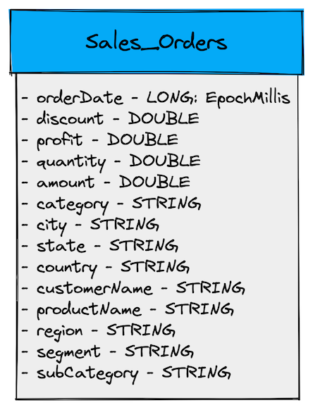
We will use a sales orders use case for this exercise.

The Use Case, The Business, and Technical KPIs:

Consider an omni-channel e-commerce platform that captures sales orders (the operational data) from multiple channels.

All orders get stored in a transactional datastore. All that operational data makes its way into the analytical system (either through an ETL/Batch process or a real-time stream).

A user-facing application connects to the analytical system and provides a 360-degree view of business metrics and get actionable insights.

Business KPIs / Insights:

• How is the daily order rate tracking?
• Which country is the biggest contributor to my revenue?
• Can I drill down by a specific dimension: region, segment, country, state, etc.?
• Which product category is most popular?
• Is there a spike in checkout error rate in the last 15 minutes?
• If so, is there a specific dimension that is causing the spike?
• How often did it happen that a user was interested in buying the product, but it was already sold out?

Technical KPIs:

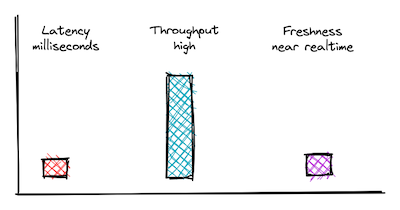
1. Latency: Since this is a user-facing application, sub-second latency is critically important.
2. Data Freshness: Some of the insights are time sensitive; A dropping order rate results in a direct loss in revenue. So the sooner we get the insight, the sooner we can act on it. Data freshness in near real-time is essential for this use case.
3. Throughput: Throughput support needed for this use case is low to start with. However, there are plans to extend the user-facing application to external users and provide the end user (the consumer of the platform) with some meaningful insights. Keeping that in mind, we want the system to support a throughput of up to 200 QPS.

Pinot Table and Schema Design Framework:

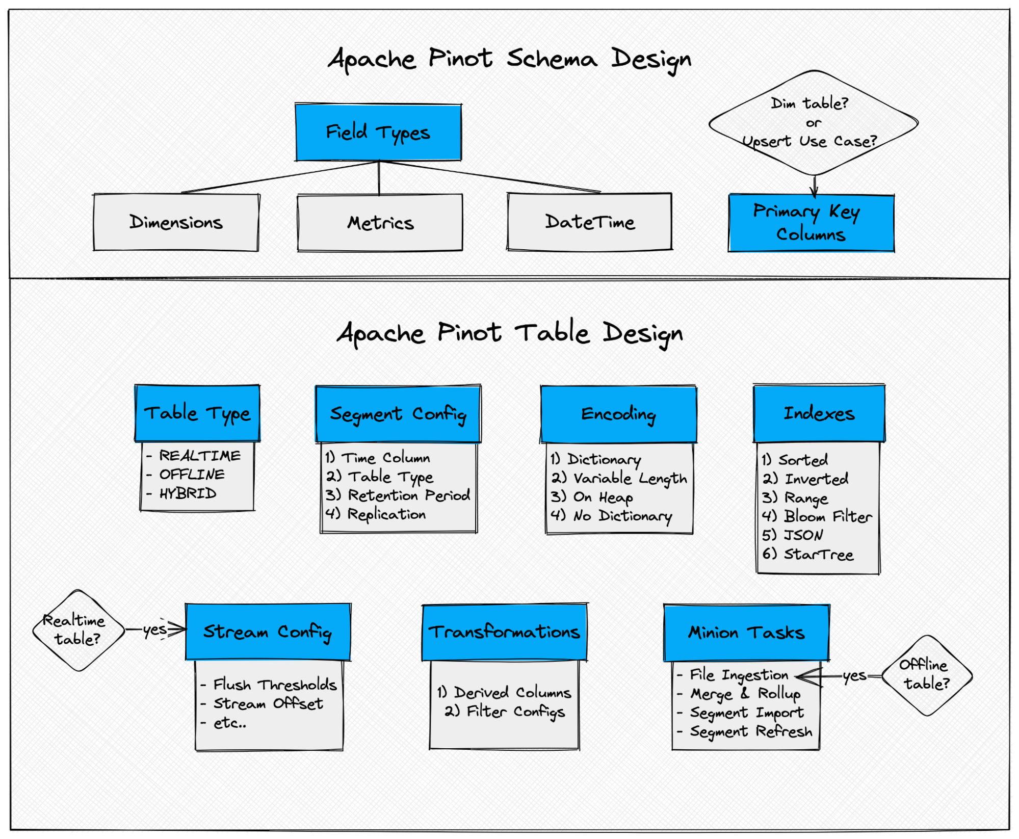
The diagram below outlines a systematic framework that can be used to design a Pinot table.

Schema Design:

First and foremost, let’s determine appropriate pinot field types (Dimension, Metric, or Datetime) for each input column.

1. DateTime Fields

DateTime Fields have three parts:

1. Data Type – The Pinot Data Type you want to store the value for this field in.
2. Format – The format in which the datetime value is present.
3. Granularity – The granularity in which the column is bucketed.

More details can be found in this pinot official doc.

Derived Columns:

Let’s take a quick detour to understand what a derived column in Apache Pinot is. Often, the user does not have control over the input data format. With derived columns and transform functions in Pinot, you can transform the input data into a format and granularity best suited for your use case. We will discuss the benefit of doing this in more detail in the transform config section.

In this case, the input column orderDate has the date in milliseconds.

This use case needs support to perform aggregations at day and minute level granularities (daily aggregates, error rate per minute, etc…). For instance, business executives want visibility into the daily order and revenue rates over the last 30 days. We also want to transform the date into a human readable format so that we don’t have to do this additional “decoration” at query time or down the stream.

We have defined three DateTime derived columns as follows:

1. orderDateEpochMillis : stores the original order date received in LONG format and granularity in MILLISECONDS .
2. orderDateEpochMinutes : stores the order date in LONG format and granularity in 15:MINUTES . All orders received in a 15-minute window are bucketed together.
3. orderDateStr : store the order date in yyyy-MM-dd string format with granularity in DAYS.

"dateTimeFieldSpecs": [  { 
 "name": "orderDateEpochMills", 
 "dataType": "LONG", 
 "format": "1:MILLISECONDS:EPOCH", 
 "granularity": "1:MILLISECONDS" 
 }, 
 { 
 "name": "orderDateEpochMinutes", 
 "dataType": "LONG", 
 "format": "1:MINUTES:EPOCH", 
 "granularity": "15:MINUTES" 
 }, 
 { 
 "name": "orderDateStr", 
 "dataType": "STRING", 
 "format": "1:DAYS:SIMPLE_DATE_FORMAT:yyyy-MM-dd", 
 "granularity": "1:DAYS" 
 } 
] 

2. Metric Fields

Metric fields are the fields on which you intend to apply aggregate functions, usually some numeric value.

"metricFieldSpecs": [  { 
 "name": "discount", 
 "dataType": "DOUBLE" 
 }, 
 { 
 "name": "profit", 
 "dataType": "DOUBLE" 
 }, 
 { 
 "name": "quantity", 
 "dataType": "INT" 
 }, 
 { 
 "name": "amount", 
 "dataType": "DOUBLE" 
 } 
]

3. Dimension Fields

Dimension fields are the fields that you will use to slice and dice (filter predicates) the data and aggregate metrics.

"dimensionFieldSpecs": [  { 
 "name": "category", 
 "dataType": "STRING" 
 }, 
 { 
 "name": "city", 
 "dataType": "STRING" 
 }, 
 { 
 "name": "country", 
 "dataType": "STRING" 
 }, 
 { 
 "name": "customerName", 
 "dataType": "STRING" 
 }, 
 { 
 "name": "productName", 
 "dataType": "STRING" 
 }, 
 { 
 "name": "region", 
 "dataType": "STRING" 
 }, 
 { 
 "name": "segment", 
 "dataType": "STRING" 
 }, 
 { 
 "name": "state", 
 "dataType": "STRING" 
 }, 
 { 
 "name": "subCategory", 
 "dataType": "STRING" 
 } 
]

4. Primary Key Columns (optional)

If your use case requires support for “upserts” or if you are creating a “dimension” table (typically used to support a lookup join use case), you will need to define the primary key column(s).

Table Design:

1. Table >> Determine Table Type

Now that schema design is ready, let’s move on to the table configuration. First, determine the table type for your table: REALTIME, OFFLINE, or HYBRID (BOTH).

We will create a hybrid table for this use case – i.e.: both real-time and offline tables.

2. Segment Config:

a. Determine the Time Column

Time column is used for determining the time boundary and managing the life cycle of data stored in pinot segments.

Note: There can only be ONE time column for a given Pinot Table.

For this use case, we will use orderDateEpochMillis as a Time Column.

b. Determine replication factor for your pinot segments

Configure the replication factor for your segments. For Production / high availability environments, the recommendation is to use a replication of at least 3, so the system can still serve data even if one or more copies are unavailable.

c. Determine retention period for your pinot segments

If your use case requires infinite retention then you can skip this step.

Configure the retention period for your Pinot segments. For Real time tables, typically this number is low (a few days), and for offline tables this number is relatively high.

For this use case, we will configure the retention period for the real time table to be 3 days and for the offline table to be 60 days. Please note that you can also consider using Managed Offline flows (using Minions) to automatically move data from RealTime Table to Offline table instead of using an offline push job.

Segment Config:

"segmentsConfig": {  "replication": "1", 
 "schemaName": "SalesOrderData", 
 "retentionTimeUnit": "DAYS", 
 "retentionTimeValue": "60", 
 "replicasPerPartition": "1", 
 "timeColumnName": "orderDateEpochMillis" 
}

3. Column Encoding

Choose an appropriate column encoding scheme for each column. More details are in the official docs here.

Fixed Length Dictionary:

• use on low cardinality columns.

Var Length Dictionary

• use on low cardinality columns with outliers (where string lengths vary a lot).
• applicable only for string and byte types.
• For all low cardinality dimension columns, we used Variable Length Dictionary Encoding.

"tableIndexConfig": {  "varLengthDictionaryColumns": [ 
 "customerName", 
 "productName", 
 "region", 
 "segment", 
 "subCategory", 
 "category", 
 "city" 
 ] 
}

On-heap Dictionary:

• avoids deserialization and hence gives performance boost.
• use with caution as this can cause out-of-memory issues.
• For country and state dimension columns which were very low cardinality, we used an On-heap dictionary.

"tableIndexConfig": {  "onHeapDictionaryColumns": [ 
 "country", 
 "state" 
 ] 
}

No Dictionary:

• use on high cardinality columns whether dictionary lookup becomes an unnecessary overhead.
• Most of the metric columns fall in this category.

"tableIndexConfig": {  "noDictionaryColumns": [ 
 "discount", 
 "profit", 
 "quantity", 
 "amount" 
 ] 
}

4. Indexes

Indexes are the key aspect of any schema design. Choosing right indexes for dimension and datetime fields is an important exercise which when done right, helps optimize / improve query performance tremendously.

Let’s start with inverted indexes. Frequently used predicate columns are great candidates for inverted indexes.

Sorted column – Sorted Inverted Index

First, identify the sort column for your Pinot table.

A pinot table can have only ONE sort column .

The most frequently used predicate column with low cardinality should be used for applying sorted inverted index .

One of the key use cases for the Sales Orders example is to find orders by a specific date. So let’s use orderDateStr as a sorted column so that we can take advantage of compression as well as data locality on this column.

"tableIndexConfig": {  "sortedColumn":["orderDateStr"], 
 … 
}

Determine inverted index columns – Bitmap Inverted Index

Next, identify if there are any low cardinality columns. Using an inverted index on such columns will help achieve a great degree of compression.

"tableIndexConfig": {  "invertedIndexColumns": [ 
 "customerName", 
 "productName", 
 "region", 
 "segment", 
 "subCategory", 
 "category", 
 "city", 
 "country", 
 "state", 
 "orderDateStr" 
 ], 
 … 
}

More details can be found in Pinot official docs here.

Determine range index columns – Range Index

Range Indexes are good for scenarios where you want to apply a range predicate on metric/timestamp columns with high cardinality (i.e.: they have a large number of unique values).

Example: Time-series queries. How is the daily revenue rate trending over the last x days?

"tableIndexConfig": {  "rangeIndexVersion": 2, 
 "rangeIndexColumns": [ 
 "orderDateStr" 
 ], 
 … 
}

Raw Value Forward Index

Now, let’s identify any remaining columns that are high cardinality and might be adversely affected by the default index (dictionary encoded forward index). The Raw Value Forward Index is the way to go for such columns.

For this use case, we have Description , a high cardinality column.

"tableIndexConfig": {  "noDictionaryColumns": [ 
 "discount", 
 "profit", 
 "quantity", 
 "amount" 
 ], 
 … 
}

Determine StarTree index – StarTree Index

StarTree Index builds aggregates at ingestion time, thereby helping avoid expensive aggregation compute at query time. Queries that compute aggregations metrics over a large data set by slicing and dicing across different dimensions will significantly improve performance with StarTree Index.

Sample Query:

SELECT  country, 
 state, 
 city, 
 Count(*) total_orders, 
 SUM(sales) total_revenue 
FROM 
 SalesOrder 
WHERE 
 orderDateStr >= ‘2022-08-01’ AND orderDateStr <= ‘2022-08-31’’ 
GROUP BY 
 country, state, city 
ORDER BY 
 orderDateStr

StarTree Index:

"tableIndexConfig": {  "starTreeIndexConfigs": [{ 
 "dimensionsSplitOrder": [ 
 "orderDateStr", 
 "city", 
 "state", 
 "country" 
 ], 
 "skipStarNodeCreationForDimensions": [], 
 "functionColumnPairs": [ 
 "COUNT__*", 
 "SUM__Price", 
 "SUM__Quantity" 
 ], 
 "maxLeafRecords": 10000 
 }], 
 … 
}

Note: Dimensions specified in dimesionsSplitOrder should be in descending order of cardinality to optimize index performance.

Dictionary Encoded Forward Index (Default)

All other columns that are not listed in the specialized indexes above will automatically get the default indexing scheme which is a dictionary-encoded forward index with bit compression .

5. Table >> Define the Stream Configuration (applicable to Real-time Tables only)

For real-time tables, we need to specify Kafka topic details in stream config. Apart from standard Kafka configs, a few additional pinot configs can be configured. These configs provide knobs to control the number and size of pinot segments.

Configure Segment Flush Threshold:

This config provides knobs to control the number and size of generated segments. By default, segments continue to consume data until the configured segment flush threshold time (default 6h) or segment flush threshold size (default 100 MB), whichever occurs first, is reached. At that point, the segment gets flushed out from memory to deepstore.

Configure Kafka consumer offset reset

This config defines whether to start consumption from the smallest offset (meaning consume all the data starting from the oldest available) or the largest offset (which means consume only the latest/fresh data that is arriving.

Stream config:

"streamConfigs":{
  ...

    "stream.kafka.sasl.mechanism": "SCRAM-SHA-512",

     "stream.kafka.decoder.prop.format": "JSON",

    "bootstrap.servers": "<SERVER_HOST>:<PORT>",

    "stream.kafka.password": "<PASSWORD>",

    "key.serializer": "org.apache.kafka.common.serialization.ByteArraySerializer",

    "stream.kafka.security.protocol": "SASL_SSL",

    "security.protocol": "SASL_SSL",

    "stream.kafka.decoder.class.name": "org.apache.pinot.plugin.inputformat.json.JSONMessageDecoder",

     "streamType": "kafka",

    "stream.kafka.username": "<USER_NAME>",

    "value.serializer": "org.apache.kafka.common.serialization.ByteArraySerializer",

     "sasl.mechanism": "SCRAM-SHA-512",

    "sasl.jaas.config": "org.apache.kafka.common.security.scram.ScramLoginModule required \n username=\"<USER_NAME>\" \n password=\"<PASSWORD>\";",

    "stream.kafka.consumer.type": "LOWLEVEL",

    "stream.kafka.broker.list": "<BROKER_HOST>:<PORT>",

    "realtime.segment.flush.threshold.rows": "1400000",

    "realtime.segment.flush.threshold.time": "24h",

    "realtime.segment.flush.threshold.segment.size": "200M",

    "stream.kafka.consumer.factory.class.name": "org.apache.pinot.plugin.stream.kafka20.KafkaConsumerFactory",

    "stream.kafka.consumer.prop.auto.offset.reset": "smallest",

    "stream.kafka.topic.name": "<TOPIC_NAME>"

    ...

}

6. Table >> Ingestion Configuration (optional):

This is where you can configure filters and transformations that you want to apply on the input data before it gets into your Pinot cluster.

Filter:

Pinot, as your OLAP data store, should host only gold-quality data. It is generally a good practice to eliminate unwanted or bad data values (such as null or empty records). However, there could be scenarios where you don’t have control over the source. In such cases, you can filter out such records by applying filter config, so they don’t get ingested.

More details can be found here.

The input source could potentially have the orderDateSinceEpochMillis field with a 0 value. Since an epoch timestamp with value 0 does not make sense, we can add a filter function to eliminate such events from entering into Pinot:

Filter config:

"ingestionConfig": {
     "filterConfig": {

          "filterFunction": "Groovy({order_date == 0}, order_date)"

      }

}

Column Transformation:

You can also apply ingestion time transformations on individual columns or create derived columns to store data in the desired transformed format that can benefit performance at query runtime.

More details can be found here.

In this example, we are creating two derived columns with respective transformFunctions which are self-explanatory.

Transform config:

"ingestionConfig": {
      "transformConfigs": [{

          "columnName": "orderDateEpochMillis",

          "transformFunction": "FromEpochDays(order_date)"

        },

        {

          "columnName": "orderDateEpochMinutes",

          "transformFunction": "toEpochMinutes(FromEpochDays(order_date))"

        },

        {

          "columnName": "orderDateStr",

          "transformFunction": "toDateTime(FromEpochDays(order_date), 'yyyy-MM-dd')"

        }]

    }

7. Minion Task (Optional)

File Ingestion Task: (Applicable to Offline tables only)

Note: This is a StarTree proprietary feature.

You can configure FileIngestionTask to set up ingestion from a batch source (such as Amazon S3 Bucket) at a periodic frequency of your choice. More details about FileIngestionTask can be found here.

FileIngestionTask provides the following knobs to control the ingestion speed. Depending on the provisioned / available capacity for minion workers, you can configure knobs to maximize resource utilization and ingestion speed.

StarTree Cloud’s Minion Autoscaling feature completely eliminates the operational overhead of monitoring and managing workers. When an ingestion task is triggered, Minion workers scale automatically as needed up to a configurable maximum number. As the sub-tasks complete, minion workers scale down as well.

A few useful configs:

• tableMaxNumTasks = total number of subtasks to generate per table.

• taskMaxDataSize = max amount of data to be processed by one task.

• taskMaxNumFiles = max number of files each sub-task can process / ingest from.

• push.mode = metadata <- recommended config; reduces controller memory pressure / overhead related to uploading segments.

"task": {
      "taskTypeConfigsMap": {

        "FileIngestionTask": {

          "schedule": "0 20 * ? * * *",

          "inputDirURI": "s3://<BUCKET_PATH>",

          "input.fs.prop.region": "us-east-1",

          "input.fs.className": "org.apache.pinot.plugin.filesystem.S3PinotFS",

          "input.fs.prop.secretKey": "<SECRET_KEY>",

          "input.fs.prop.accessKey": "<ACCESS_KEY>", 

          "taskMaxDataSize": "2G",

          "tableMaxNumTasks": "200",

          "maxNumRecordsPerSegment": "50000000",

          "inputFormat": "PARQUET",

          "includeFileNamePattern": "glob:**/*events/**.parquet",

          "push.mode": "metadata"

        }

      }

}

Minion Merge Rollup Task: 

This segment optimization task merges smaller segments into a larger one.

More details here.

Note: As of Jan 2022, this applies to offline tables only.

MergeRollupTask config:

"task": {
  "taskTypeConfigsMap": {

    "MergeRollupTask": {

          "1day.mergeType": "concat",

          "1day.bucketTimePeriod": "1d",

          "1day.bufferTimePeriod": "1d"  

     }

   }

}

Managed Offline Flow > RealTime to Offline Segments Task: 

If you create a hybrid table, you can configure the following automated task – RealtimeToOfflineSegmentsTask – which can run periodically to move all eligible segments from Realtime to Offline table.

More details here.

RealtimeToOfflineSegmentsTask config:

"task": {
  "taskTypeConfigsMap": {

    "RealtimeToOfflineSegmentsTask": {

      "bucketTimePeriod": "1h",

      "bufferTimePeriod": "1h",

      "schedule": "0 * * * * ?"

    }

  }

}

SegmentRefreshTask

"task": {
  "taskTypeConfigsMap": {

    "SegmentRefreshTask": {

          "bucketTimePeriod": "1d",

          "tableMaxNumTasks": "100",

          "maxNumRecordsPerTask": "50000000",

          "maxNumRecordsPerSegment": "50000000",

          "skipSegmentIndexCheck": "true",

          "push.mode": "metadata",

          "schedule": "0 */5 * * * ?"

        }

  }

}

Important Note: Please note that the minion tasks will not run unless the controller is configured to schedule the task frequency config. More details in this doc.

In conclusion, the above framework can be easily expanded to cover other additional use case scenarios as well as utilizing other Apache Pinot features. Further, depending on the query throughput/SLA requirements users might also consider utilizing advanced performance tuning strategies in Apache Pinot.