StarTree benchmark demonstrates breakthrough performance for query on Iceberg data lakes

Imagine you have a massive library with 12.2 billion books  stored in a giant warehouse (Amazon S3). You can’t move the books. You can’t reprint them in a different format. But you still need to find answers fast: “How many books mention topic X in the last hour?” or “Show me a breakdown by author for this category.“

That’s essentially the challenge modern data teams face. Petabytes of data sitting as Parquet files on S3 – open, portable, cost-effective but querying it at interactive speeds? That’s where things get tricky.

StarTree recently introduced StarTree Iceberg Tables — a feature that extends Apache Pinot’s lightweight indexes to accelerate queries on data stored in open table and file formats. Think of it like adding a card catalog to that giant library — the books don’t move, but now you can find what you need in seconds instead of walking every aisle.

We wanted to put this to the test. How do Iceberg Tables from StarTree compare against Trino and ClickHouse OSS — two popular engines that can also query Iceberg data in a fair, head-to-head benchmark?

Here’s what we found:

Dataset

We used a synthetic observability dataset modeled after real-world telemetry — the kind of wide-column, time-series metrics you’d see in monitoring and APM platforms.

Property	Value
Total Rows	~12.2 billion
Total Size on S3	770 GB
Storage Format	Apache Parquet
Storage Location	Amazon S3 (us-west-1)
Schema Type	Wide column (metrics with dimensions map)
Key Columns	org_id, metric, resolution, logical_timestamp, sum_rollup, latest_rollup, dimensions (MAP)

System Configuration

Getting a fair benchmark right is harder than running the benchmark itself. Each of these systems has its own sweet spot, and we wanted each one configured at its best. Here’s what we did and why

Hardware & Infrastructure (Identical Across Systems)

Before diving into system-specific configs, one critical detail: every system ran on identical hardware. Same instance types, same cluster topology, same disk sizes. No system got a resource advantage.

Role	Instance Type	Specs	Disk	Count
Coordinator	AWS EC2 m7g.xlarge	16 GB RAM, 4 vCPUs	128 GB	1
Workers / Servers	AWS EC2 r6gd.4xlarge	128 GB RAM, 16 vCPUs	800 GB	4

The naming varies by system (Trino calls them “coordinator” and “workers”, ClickHouse has its “coordinator” and “servers”, Pinot uses “controller” and “servers”) but the topology is the same: 1 coordinator node for planning and routing, 4 worker nodes for data processing and S3 access.

StarTree (v14.0) using Iceberg Tables

StarTree builds on Apache Pinot for a fundamentally different approach from Trino and ClickHouse. To understand why, a quick analogy helps.

Imagine those 12.2 billion rows are books on shelves. Trino and ClickHouse look at the shelf labels (Iceberg metadata) to figure out which shelves to skip. That’s useful because you avoid entire aisles you don’t need. But once you pick a shelf, you still have to flip through every book on it.

Pinot can do something different. It builds an actual index — like a library card catalog — that tells you exactly which books on which shelves have what you’re looking for. You go straight to the right pages without flipping through anything.

Technically, here’s what happens:

• The Parquet files stay on S3 untouched. No copies, no format conversion.
• Pinot builds index-only segments: inverted indexes for exact lookups, range indexes for time-range scans, and sorted indexes for ordered access. These indexes reference the original Parquet columns as the data source. These indexes can be stored remotely, but can also reside locally when specifically pinned.
• At query time, Pinot consults its indexes first to identify exactly which rows match, then reads only the necessary column data from Parquet. The indexes do the heavy lifting and the Parquet files just serve the data.

The result: Pinot can skip irrelevant rows at the individual document level, not just the file or partition level. And all of this happens without duplicating the data.

Trino (v476) using Iceberg Connector

For optimal query performance, we utilized optimized Iceberg tables configured with proper, granular partitioning, improving upon the initial single-partition (org_id) setup.

CREATE TABLE iceberg_data."st-database"."iceberg_benchmark_partitioned"
WITH (
  format = 'PARQUET',
  partitioning = ARRAY['org_id', 'day(event_date)'],
  sorted_by = ARRAY['org_id', 'event_date']
) AS
SELECT *, from_unixtime(logical_timestamp / 1000) AS event_date
FROM s3_data."st-database"."iceberg-dataset";Code language: SQL (Structured Query Language) (sql)

This gives Trino what it needs: Iceberg manifest files that enable partition pruning (skip entire directories of files that can’t match) and column-level min/max statistics (skip individual files whose value ranges don’t overlap with the query predicates).

Is this still a fair comparison? Yes because real-world customers would typically already have their data partitioned this way. We gave Trino every reasonable advantage.

ClickHouse OSS (v26.2.5) using icebergS3Cluster

ClickHouse was the trickiest to configure fairly. Here’s why:

The most common ClickHouse OSS deployment uses MergeTree tables, its native columnar format heavily optimized for fast queries. But MergeTree converts Parquet into ClickHouse’s own format. That’s not querying data on S3; that’s ingesting it. It would be like comparing Pinot’s local tables (where data is fully indexed and stored in Pinot’s format) rather than external tables. Not apple-to-apple.

On the other end, ClickHouse’s s3Cluster() function reads raw Parquet directly from S3 with no metadata at all — no partition pruning, no statistics. That unfairly penalizes ClickHouse, since it’s essentially doing full scans.The right middle ground is icebergS3Cluster(). This is ClickHouse’s Iceberg integration that queries the exact same Iceberg tables we set up for Trino, utilizing same partition pruning, and same column statistics, and same Parquet data on S3.

Queries

We picked four queries that cover the most common analytical patterns in observability workloads. Each one tests something different.

Q1: Filtered Count
A broad count across millions of rows, filtered by resolution and a one-hour time window. This tests raw scan throughput.

SELECT COUNT(*)
FROM iceberg_table
WHERE resolution = 15000
  AND logical_timestamp >= 1754229600000 - 3600000
  AND logical_timestamp <= 1754229600000

Q2: Selective Aggregation
A targeted SUM with tight filters on metric, org_id, resolution, and time range. This tests how well each system narrows down to a small set of matching rows.

SELECT SUM(sum_rollup)
FROM iceberg_table
WHERE metric = 'tk_cache'
  AND org_id = 184833768
  AND resolution = 15000
  AND logical_timestamp >= 1754229600000 - 3600000
  AND logical_timestamp <= 1754229600000Code language: JavaScript (javascript)

Q3: Time-Bucketed Aggregation
A GROUP BY with time bucketing which is the classic pattern behind every time-series dashboard chart.

SELECT dateTrunc('second', logical_timestamp) AS time_bucket,
       AVG(latest_rollup)
FROM iceberg_table
WHERE metric = 'tk_cache'
  AND org_id = '184833768'
  AND resolution = 15000
  AND logical_timestamp >= 1754229600000 - 3600000
  AND logical_timestamp <= 1754229600000
GROUP BY dateTrunc('second', logical_timestamp)
ORDER BY time_bucketCode language: PHP (php)

Q4: Map Column Aggregation
This filters on a nested map key (dimensions['node']), groups by another map key (dimensions['service']), and orders by the result. Semi-structured data access is notoriously difficult to optimize in columnar formats.

SELECT dimensions['service'] AS service,
       SUM(sum_rollup) AS total_value
FROM iceberg_table
WHERE metric = 'tk_cache'
  AND org_id = '184833768'
  AND resolution = 15000
  AND dimensions['node'] = 'xyz'
  AND logical_timestamp >= 1754229600000 - 360000
  AND logical_timestamp <= 1754229600000
GROUP BY dimensions['service']
ORDER BY total_value DESCCode language: PHP (php)

Implementation

We used Apache JMeter with all four queries in a single thread group, running in a loop. Single-threaded, sequential execution — measuring per-query latency without concurrency noise.

Parameter	Without Cache	With Cache
Warmup Runs	5–10 queries per system	5–10 queries per system
Benchmark Loops	100	100
Threads	1 (sequential)	1 (sequential)

Every system was warmed up before recording. The numbers you see below are all post-warmup.

A Note on Pinning and Caching

To minimize S3 reads, Trino and ClickHouse OSS use a traditional File System (FS) cache for previously read data. StarTree utilizes two independent layers: Index Pinning (preloading index files to disk to prevent remote reads) and a Disk Page Cache (for Parquet data pages).

To accurately isolate the performance impact of each layer, we benchmarked Pinot across three distinct modes: no local storage, index pinning only, and index pinning combined with the disk page cache.

Results

Without Cache

These are cold queries — every execution reads from S3. No local caching for any system.

Query	StarTree Avg (ms)	Trino Avg (ms)	ClickHouse Avg (ms)
Q1 – Filtered Count	491	10,237	19,200
Q2 – Selective Aggregation	515	4,886	6,634
Q3 – Time-Bucketed Agg	645	5,486	7,451
Q4 – Map Column Agg	2,390	9,219	26,973

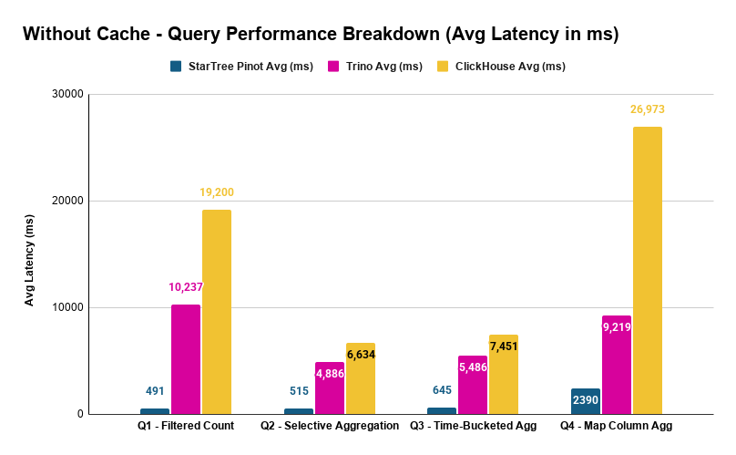
The speedups are dramatic:

Query	Pinot vs Trino	Pinot vs ClickHouse OSS
Q1	20.8x faster	39.1x faster
Q2	9.5x faster	12.9x faster
Q3	8.5x faster	11.6x faster
Q4	3.9x faster	11.3x faster

With Cache

Here we compare each system’s cached performance. For Trino and ClickHouse, that’s FS cache. For Pinot, we show index cache only — indexes pinned in local disk, Parquet data still read from S3 — as it delivered the best overall results (more on the disk page cache below).

Query	StarTree Avg (ms)	Trino Avg (ms)	ClickHouse Avg (ms)
Q1 –  Filtered Count	287	4,076	4,103
Q2 – Selective Aggregation	483	1,981	2,972
Q3 – Time-Bucketed Agg	615	2,213	3,038
Q4 – Map Column Agg	382	6,624	14,007

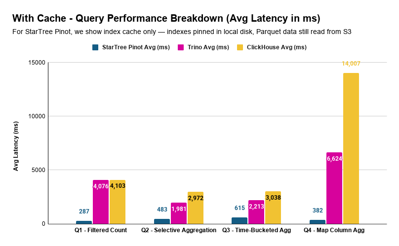
Query	Pinot vs Trino	Pinot vs ClickHouse
Q1	14.2x faster	14.3x faster
Q2	4.1x faster	6.2x faster
Q3	3.6x faster	4.9x faster
Q4	17.3x faster	36.7x faster

With index pinning, Pinot answers every query in under 650 milliseconds. The most complex query – Q4, the map column aggregation that takes ClickHouse OSS 14 seconds and Trino 6.6 seconds while Pinot handles it in 382 milliseconds.

Pinot’s Caching Layers

Pinot’s two caching layers have very different effects depending on the query pattern:

Query	No Cache (ms)	Index Pinning Only (ms)	Index Pinning + Disk Page Cache (ms)
Q1	491	287	282
Q2	515	483	1,211
Q3	645	615	1,651
Q4	2,390	382	457

Index pinning alone is the clear winner for Q2 and Q3 — adding disk page cache actually makes them slower (515ms → 1,211ms for Q2, 645ms → 1,651ms for Q3). Q4, on the other hand, benefits from both layers (2,390ms → 457ms).

The takeaway: for selective, index-accelerated queries, Pinot’s indexes are so effective at reducing data access that additional data caching adds overhead rather than value. The indexes themselves are the primary accelerator. For queries that touch expensive-to-read data like map columns, disk page caching provides additional benefit.

For selective, index-accelerated queries, Pinot’s indexes are so effective at reducing data access that additional data caching adds overhead rather than value.

Full Breakdown

StarTree (Pinot): Iceberg Tables

Query	Avg (ms)	P90 (ms)	P95 (ms)
Q1	491	523	545
Q2	515	554	564
Q3	645	667	709
Q4	2,390	2,418	2,440
Q1 – index pinning	287	296	320
Q2 – index pinning	483	508	538
Q3 – index pinning	615	643	679
Q4 – index pinning	382	385	393
Q1 – index pinning + disk page cache	282	288	305
Q2 – index pinning + disk page cache	1,211	1,260	1,292
Q3 – index pinning + disk page cache	1,651	1,683	1,711
Q4 – index pinning + disk page cache	457	459	507

Trino (v476)

Query	Avg (ms)	P90 (ms)	P95 (ms)
Q1	10,237	10,658	11,008
Q2	4,886	5,234	5,257
Q3	5,486	5,648	5,723
Q4	9,219	9,492	9,602
Q1 – with FS cache	4,076	4,611	4,764
Q2 – with FS cache	1,981	2,184	2,256
Q3 – with FS cache	2,213	2,364	2,630
Q4 – with FS cache	6,624	6,847	6,988

ClickHouse OSS (v26.2.5)

Query	Avg (ms)	P90 (ms)	P95 (ms)
Q1	19,200	19,395	19,408
Q2	6,634	6,712	6,743
Q3	7,451	7,532	7,571
Q4	26,973	27,081	27,146
Q1 – with FS cache	4,103	4,293	4,318
Q2 – with FS cache	2,972	3,144	3,187
Q3 – with FS cache	3,038	3,233	3,294
Q4 – with FS cache	14,007	14,458	14,679

Observations

Pinot’s Iceberg Tables are in a different league

The numbers speak plainly. Without any caching, Pinot is 9–39x faster than ClickHouse OSS and 4–21x faster than Trino depending on the query. With caching, Pinot is 5–37x faster than ClickHouse OSS and 4–17x faster than Trino.

To put that in perspective: ClickHouse OSS takes 19 seconds for Q1. Trino takes 10 seconds. Pinot takes 491 milliseconds — well under a second. That’s not an incremental improvement. It’s an order-of-magnitude difference.

The gap is widest on Q1 (broad scan) and Q4 (map columns) — exactly the query patterns where Pinot’s index-based approach has the most room to outperform metadata-only pruning. And it’s narrowest on Q2 and Q3 (selective aggregations), where tight predicates already reduce the data each system needs to process.

Trino consistently outperforms ClickHouse

Even though both Trino and ClickHouse OSS use the same Iceberg metadata on the same Parquet files, Trino is faster across every query:

• Q1: 10.2s vs 19.2s — 1.9x faster
• Q2: 4.9s vs 6.6s — 1.4x faster
• Q3: 5.5s vs 7.5s — 1.4x faster
• Q4: 9.2s vs 27.0s — 2.9x faster

This makes sense. Trino’s Iceberg connector has been battle-tested for years — its query planner knows how to aggressively push predicates into Iceberg’s metadata layer. ClickHouse’s icebergS3Cluster() is a newer capability, and the gap shows most clearly on Q4 (map columns) where query planning matters the most.

Map columns (Q4) are where systems diverge the most

Q4 is the outlier in every comparison. It filters on dimensions['node'] and groups by dimensions['service'] — nested key-value access inside a MAP column.

Here’s why this is so hard: when data is stored as Parquet, map columns are encoded as repeated key-value structures. Unlike top-level columns where min/max statistics can help skip entire row groups, map columns offer no such shortcut. The engine essentially has to scan the full map data to check if a particular key has a particular value.

ClickHouse OSS at ~27 seconds without cache on Q4 suggests it’s doing something close to a full scan of the map column. Trino at ~9 seconds handles it better but still takes roughly 2x its non-map queries. Pinot? 2.4 seconds without cache, 382 milliseconds with index pinning. That’s because Pinot extracts map keys into indexed columns during segment creation — filtering on dimensions['node'] becomes no different from filtering on a regular column like org_id. The map column penalty that plagues Trino and ClickHouse OSS simply doesn’t exist.

Pinot’s indexes eliminate work

Pinot’s query response includes statistics that show exactly how much work its indexes eliminate. Here’s what each query actually touched out of the 12.2 billion total rows:

Query	Total Rows	After Segment Pruning	After Index Filtering	Data Eliminated
Q1 — Filtered Count	12.2B	3.91B	811M	93.4%
Q2 — Selective Agg	12.2B	3.91B	80M	99.3%
Q3 — Time-Bucketed Agg	12.2B	3.91B	80M	99.3%
Q4 — Map Column Agg	12.2B	3.63B	25	99.9999998%

Pinot filters data in two stages. First, segment pruning skips entire segments whose metadata (time ranges, partition values) can’t match the query — this is conceptually similar to what Trino and ClickHouse do with Iceberg manifest files. For Q1–Q3, this eliminates ~68% of the data.

The second stage is where Pinot pulls ahead: index filtering within the remaining segments. Inverted indexes on metric, org_id, and resolution narrow Q2/Q3 from 3.91 billion to 80 million matching rows — a 97.9% reduction that Trino and ClickHouse can’t achieve because they lack row-level indexes.Q4 is the most striking. The dimensions[‘node’] = ‘xyz’ filter — applied through an inverted index on the extracted map key — reduces 3.63 billion candidate rows down to exactly 25 matching documents. That’s a selectivity of 0.0000002%. No amount of file-level or partition-level pruning can come close to this kind of precision. It’s the difference between checking every book on a shelf and looking up exactly 25 entries in a card catalog.

Caching helps everyone — but reveals where the real bottleneck is

With caching enabled, all systems get faster since repeated S3 reads come from local disk:

Query	Trino Improvement	ClickHouse OSS Improvement	Pinot Improvement
Q1	10.2s → 4.1s (2.5x)	19.2s → 4.1s (4.7x)	491ms → 287ms (1.7x)
Q2	4.9s → 2.0s (2.5x)	6.6s → 3.0s (2.2x)	515ms → 483ms (1.1x)
Q3	5.5s → 2.2s (2.5x)	7.5s → 3.0s (2.5x)	645ms → 615ms (1.0x)
Q4	9.2s → 6.6s (1.4x)	27.0s → 14.0s (1.9x)	2,390ms → 382ms (6.3x)

A few things stand out.

Pinot benefits the least from caching on Q2 and Q3 — and that’s actually a good sign. These selective queries are already so fast (under 650ms) that there’s almost nothing left to cache. The indexes have already eliminated the bulk of the work. Caching is most useful when the system has to read a lot of data; when indexes pre-select exactly what’s needed, there’s less data to cache in the first place.

ClickHouse’s Q1 improves by 4.7x with caching — dropping from 19.2s to 4.1s, nearly matching Trino’s cached Q1 at 4.1s. That tells us something: without caching, ClickHouse’s Q1 bottleneck was primarily S3 I/O latency, not compute. Once you eliminate the I/O, the engines converge on a simple count query.But Q4 tells a different story. Even with caching, ClickHouse sits at 14 seconds while Trino is at 6.6 seconds. The I/O bottleneck is gone — what’s left is pure query execution efficiency on map column data. That 2x gap is in the engine itself, not in S3.

Low variance confirms the results are stable

Across all systems, the difference between average and P95 latency is tight — typically 5–10%. This held true across both cached and non-cached runs, meaning these aren’t noisy measurements. The numbers are stable and reproducible.

Resource efficiency – Pinot does more with less

Performance isn’t just about latency, it’s about what that latency costs in compute resources. We captured CloudWatch metrics across all three clusters during the without-cache/index-pinning benchmark runs.

Metric (Worker/Server Avg)	StarTree	Trino	ClickHouse
CPU Utilization	7.1%	31.3%	44.8%
Network In (GB)	4.2	19.3	20.5
Network Out (GB)	0.024	0.101	0.076
EBS Write (GB)	0.002	0.002	1.55

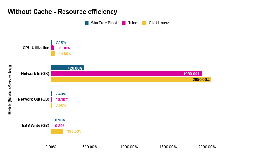
Three things jump out:

Pinot uses 4–6x less CPU. At 7.1% average CPU across four workers, Pinot is highly efficient while delivering sub-second latencies. Trino and ClickHouse sit at 31% and 45% respectively and take 5–27 seconds per query. Indexes eliminate the scan-and-filter work that dominates the other engines.

Pinot reads 5x less data from S3. Average network-in per worker is 4.2 GB for Pinot vs ~20 GB for Trino and ClickHouse. Pinot’s indexes identify exactly which Parquet row groups to fetch. The other systems, even with Iceberg partition pruning, read far more data to evaluate their predicates. Less data read means proportionally fewer S3 GET requests, a variable cost that scales directly with query volume.

ClickHouse writes significantly to disk, even without caching. At 1.55 GB average EBS writes per worker, ClickHouse spills intermediate data to disk during query processing. Pinot and Trino write essentially nothing. Under sustained workloads, these writes consume EBS IOPS and throughput budget and once you exceed gp3 baseline limits (3,000 IOPS / 125 MB/s), provisioned IOPS charges apply at $0.005/IOPS/month. This is a variable I/O cost that Pinot and Trino avoid entirely.

Cost per query – the economic case

All three systems ran on identical infrastructure. The cluster costs the same per hour regardless of which engine runs on it. The question is: how many queries does that hourly spend buy you?

Cluster cost (AWS on-demand, us-west-1):

Component	Instance	Count	$/hr	Subtotal
Coordinator	m7g.xlarge	1	$0.19	$0.19
Workers / Server	r6gd.4xlarge	4	$1.04	$4.16
Total		5		$4.35/hr

Sequential throughput (one query at a time, cycling through Q1–Q4):

Lower latency means more queries completed per hour on the same hardware. Using the average latencies from the without-cache benchmark, each loop (Q1 + Q2 + Q3 + Q4) takes:

System	Avg Time per Loop (4 queries)	Loops/hr	Queries/hr
StarTree (Pinot)	4.04s	891	3,564
Trino	29.83s	121	483
ClickHouse	60.26s	60	239

On the same cluster, Pinot serves 7.4x more queries than Trino and 14.9x more than ClickHouse every hour.

Cost per query (without cache/index-pinning):

System	$/Query	Relative Cost
StarTree (Pinot)	$0.0012	1x
Trino	$0.0090	7.4x more expensive
ClickHouse	$0.0182	14.9x more expensive

Each ClickHouse query costs nearly 15x more than a Pinot query. Trino is 7.4x more expensive. Same hardware, same data, same queries but different architecture.

And this is the conservative estimate – single-threaded, no concurrency. In production with multiple users querying simultaneously, Pinot’s 7.1% CPU utilization means the cluster has massive headroom for concurrent queries that the other systems don’t have. Trino at 31% and ClickHouse at 45% are already consuming a substantial share of available compute with just a single query stream. Scale to realistic concurrency and Pinot’s cost advantage widens further.

Beyond compute, S3 and I/O costs widen the gap. The $/query numbers above reflect only the fixed cluster cost. But S3 API charges and EBS I/O are variable costs that scale with every query  and they favor Pinot even further:

• S3 GET requests ($0.0004 per 1,000 GETs in us-west-1): Pinot’s workers read 5x less data from S3 (4.2 GB vs ~20 GB per node), which translates to proportionally fewer GET requests. At high query volumes, this adds up. A system doing 3,564 queries/hr at one-fifth the S3 requests per query has a materially lower S3 API bill than one doing 239 queries/hr at 5x the requests per query.
• EBS I/O: ClickHouse writes 1.55 GB per worker to EBS per benchmark run even with caching disabled. Across 4 workers, that’s over 6 GB of disk writes per run. Under sustained production load, this consumes EBS IOPS budget and can trigger provisioned IOPS charges. Pinot and Trino write essentially zero to EBS.
• Network bandwidth ceiling: Each r6gd.4xlarge supports up to 10 Gbps. Trino and ClickHouse consume ~20 GB of network-in per worker per run that’s 5x more than Pinot’s 4.2 GB. Under concurrent workloads, they’ll saturate network capacity sooner, forcing horizontal scale-out (more nodes, more cost) while Pinot’s cluster still has bandwidth to spare.

Pinot’s additional storage cost. Pinot’s index-only segments add 270 GB on S3 for this 770 GB dataset — a 35% storage overhead at ~$6.21/month (S3 Standard). Against the $4.35/hr cluster cost, that’s less than a 0.2% increase. And against the S3 GET request savings from reading 5x less data per query, the index storage cost pays for itself quickly at any non-trivial query volume.

Scaling Under Load (QPS Benchmark)

The latency benchmarks above measured single-threaded, sequential queries which is useful for controlled comparison, but not how production systems operate. Real workloads are concurrent: dashboards refreshing, alerts firing, analysts exploring – all at once.

We ran a separate QPS (queries per second) benchmark on Pinot using JMeter, testing each query type independently with only index pinning enabled. Starting from low QPS targets, we ramped up until the cluster reached saturation — same hardware, same data, same queries.

Q1: Filtered Count

QPS Target	QPS Achieved	Avg Latency (ms)	Avg Server CPU	Avg of Peak Server’s CPU
10	10	284	3.1%	3.5%
100	100	365	29.6%	34.3%
200	199	373	59.0%	68.1%
250	249	409	74.1%	85.4%
300	280	1,758	83.4%	96.7%

Q1 scales linearly to 249 QPS with sub-500ms latency. At 300 QPS the cluster saturates and latency spikes 4x and achieved QPS falls short of the target. Remember, this is the query that scans 811 million matching rows across 12.2 billion total and Pinot handles 249 concurrent executions per second of it.

Q2: Selective Aggregation

QPS Target	QPS Achieved	Avg Latency (ms)	Avg Server CPU	Avg of Peak Server’s CPU
10	10	351	22.7%	35.9%
30	30	539	62.4%	81.6%
100	36	5,420	74.7%	97.1%

Q3: Time-Bucketed Aggregation

QPS Target	QPS Achieved	Avg Latency (ms)	Avg Server CPU	Avg of Peak Server’s CPU
1	1	635	7.6%	16.7%
5	5	638	35.3%	72.9%
7	7	779	47.6%	94.6%
9	8	1,168	50.8%	98.2%

Q3 – GROUP BY with time bucketing and ORDER BY over 80 million rows is the most compute-intensive query in the set. Sustained throughput: 7 QPS before the hottest server saturates. Even so, 7 concurrent time-series dashboard queries per second on a 12.2 billion row dataset is notable.

Q4: Map Column Aggregation

QPS Target	QPS Achieved	Avg Latency (ms)	Avg Server CPU	Avg Broker CPU
10	10	273	0.2%	1.6%
100	100	262	1.0%	10.0%
200	200	268	1.8%	18.7%
250	249	289	2.2%	23.9%
500	498	299	4.3%	54.0%

Q4 is the most striking result in the entire benchmark. The query that takes ClickHouse 27 seconds and Trino 9 seconds? Pinot serves it at 498 QPS with sub-300ms latency. Server CPU is virtually idle at 4.3% because the indexes reduce the work to exactly 25 matching documents out of 12.2 billion. The bottleneck isn’t the data servers at all; it’s the broker (coordinator) at 54% CPU, routing and merging results.

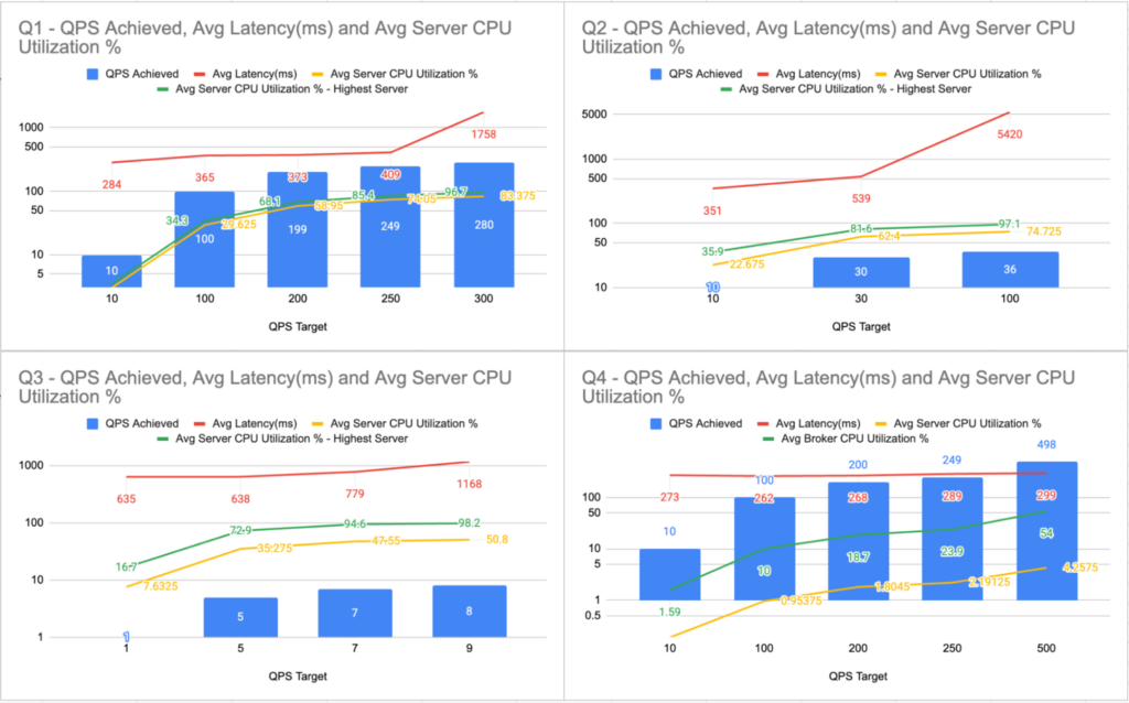
Maximum Sustainable QPS (Index Pinning Only)

Query	Max Sustained QPS	Avg Latency (ms)	Bottleneck
Q1: Filtered Count	249	409	Server CPU
Q2: Selective Aggregation	30	539	Server CPU
Q3: Time-Bucketed Agg	7	779	Server CPU
Q4: Map Column Agg	498	299	Broker CPU

All numbers above are with index pinning only – indexes pinned in local disk, Parquet data still read from S3 on every query. Each query type was tested independently – only one query type running at a time. The bottleneck varies by query pattern: broad scans (Q1–Q3) are server-CPU bound, while highly selective index lookups (Q4) shift the bottleneck to the broker.

Cost per query at scale

At maximum sustained QPS, the economics change dramatically from the sequential estimates:

Query	Max QPS	Queries/hr	$/Query at Scale	vs Sequential
Q1	249	896,400	$0.000005	240× cheaper
Q2	30	108,000	$0.00004	30× cheaper
Q3	7	25,200	$0.00017	7× cheaper
Q4	498	1,792,800	$0.0000024	500× cheaper

Even Q3, the heaviest query at scale costs only $0.00017 per query. Q4, the query that takes other engines 9–27 seconds each, costs less than a quarter of a cent per thousand queries.

Under the Hood: Why StarTree’s Approach is Different

Let’s go back to the library analogy. All three systems are querying data in the same format (Parquet) in the same warehouse (S3). The difference is how they find what they’re looking for.

Trino and ClickHouse use Iceberg metadata — essentially shelf labels. The Iceberg manifest tells them: “Files in partition org_id=184833768 are in this directory. File X has timestamps between A and B.” This lets them skip entire files (or shelves) that can’t possibly match. But once they open a file, they read through all the rows in it.

Pinot builds actual indexes — the card catalog. Inverted indexes map values back to document IDs (“these 47 rows have metric=’tk_cache'”). Range indexes map value ranges to document IDs (“these rows have timestamps in your window”). Sorted indexes allow binary search over ordered data.

The difference in granularity:

	Trino & ClickHouse	StarTree (Pinot): Iceberg Tables
What it uses	Iceberg manifests (partition info, file-level min/max)	Purpose-built indexes (inverted, range, sorted)
Skips at	File and row-group level	Individual row level
How it filters	Scan column data, apply predicate	Index lookup — go directly to matching rows
Map columns	Scan the entire map column	Indexes on extracted map keys — same speed as top-level columns

That last row is especially important. For Q4, Trino and ClickHouse have to scan through the entire map column because there’s no way to push a predicate like dimensions['node'] = 'xyz' into Parquet file statistics. Pinot, on the other hand, extracts map keys into indexed columns during segment creation — so filtering on dimensions['node'] is no different from filtering on org_id.

And all of this happens without copying the data. The Parquet files on S3 are the source of truth. Pinot’s segments are pure index metadata — lightweight structures that point back to the original data.This also explains the caching behavior we observed. When indexes are this effective at reducing data access, traditional data caching (like FS cache or disk page cache) adds less value — because there’s less data to cache. The acceleration comes from not reading data in the first place, rather than reading it faster from a local cache.

Keeping It Fair

Benchmarks published without transparency invite skepticism — and rightly so. Here’s how we made sure this comparison is defensible.

Same data, same queries. All three systems query the same Parquet data on S3 with equivalent SQL. The storage structure was optimized for each system’s requirements to ensure a fair comparison.

Same measurement. All latencies were measured end-to-end from JMeter. This captures real client-observed latency, not internal server-side execution time. Pinot’s internal timeUsedMs metric reports much lower numbers (e.g., ~19ms for Q2), but we report client-observed latency for consistency across all three systems.

Every system gets its best shot. We didn’t just throw each system at the problem — we configured each one with its best available approach for querying S3-resident data:

System	What It Uses	Data Format
StarTree (Pinot)	Index-only segments (inverted, range, sorted) over Parquet	Raw Parquet (partitioned by org_id)
Trino	Iceberg connector with partition pruning and column statistics	Optimized Iceberg Parquet (granular partitioning + metadata)
ClickHouse	icebergS3Cluster() with same Iceberg metadata as Trino	Optimized Iceberg Parquet (granular partitioning + metadata)

No proprietary format conversion. ClickHouse MergeTree was intentionally excluded because it converts Parquet into ClickHouse’s native columnar format. That would be equivalent to comparing Pinot’s local tables — not the lceberg Tables feature. Every system in this benchmark reads Parquet from S3 at query time.

Identical infrastructure. All three systems ran on the same hardware: 1 coordinator (m7g.xlarge, 16 GB RAM, 4 vCPUs, 128 GB disk) and 4 workers (r6gd.4xlarge, 128 GB RAM, 16 vCPUs, 800 GB disk each). No system got a resource advantage.

Conclusion

When data lives in Iceberg on object storage, how you query it matters enormously. This benchmark shows that the approach you choose — metadata-based pruning vs. purpose-built indexes over the same data — can mean the difference between seconds and sub-second response times.

The numbers tell a clear story:

• Raw Performance: Pinot is 9–39x faster than ClickHouse OSS and 4–21x faster than Trino without any local storage. With caching enabled, Pinot remains 5–37x faster than ClickHouse OSS and 4–17x faster than Trino.
• Sub-Second Latency: Every Pinot query completes in under 650ms with index pinning. This includes the complex map column aggregation that takes other systems 7–14 seconds.
• Drastically Lower Costs: On identical hardware, Pinot is 7.4x cheaper than Trino and 14.9x cheaper than ClickHouse ($0.0012/query vs. $0.009 and $0.018, respectively) while leaving massive CPU headroom for concurrent workloads.
• Concurrent throughput: Pinot sustains 7–498 QPS per query type on the same cluster, driving cost per query as low as $0.000005

StarTree delivers these results by doing something the other systems can’t: building lightweight, purpose-built indexes over Parquet data on S3 without moving, copying, or converting it. The Parquet files stay exactly where they are. They remain readable by every tool in the data lake ecosystem. Pinot simply adds a smart acceleration layer on top.For teams already sitting on large volumes of Parquet data in S3, this means real-time query performance without the cost and complexity of data migration.

	StarTree (Pinot)	Trino	ClickHouse
Data format on S3	Original Parquet	Iceberg Parquet	Iceberg Parquet
Acceleration	Indexes (inverted, range, sorted)	Partition pruning, column stats	Partition pruning, column stats
Data duplication	None	Iceberg metadata only	Iceberg metadata only
Cost per query (no cache)	$0.0012	$0.0090	$0.0182
Avg Server CPU	7.1%	31.3%	44.8%
Max QPS (Q1/Q4)	249 / 498	N/A	N/A

Get Started from here: Docs: Iceberg Table Onboarding via Data Portal 

Try Iceberg Tables with StarTree — powered by Apache Pinot

The best way to experience the power of StarTree with Iceberg tables is to book a demo or request a trial to run your own benchmark, on your own data, with your own queries