GapFill Function For Time-Series Datasets In Pinot

Many real-world datasets are time-series in nature, tracking the value or state changes of entities over time. The values may be polled and recorded at constant time intervals or at random irregular intervals or only when the value/state changes. There are many real-world use cases of time series data. Here are some specific examples:

• Telemetry from sensors monitoring the status of industrial equipment.
• Real-time vehicle data such as speed, braking, and acceleration, to produce the driver’s risk score trend.
• Server performance metrics such as CPU, I/O, memory, and network usage over time.
• An automated system tracking the status of a store or items in an online marketplace.

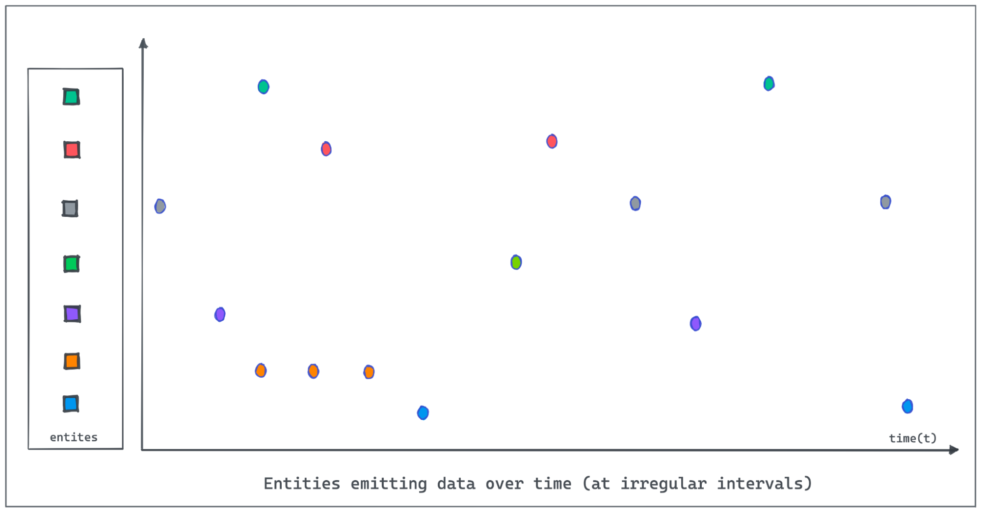
Let us use an IOT dataset tracking the occupancy status of the individual parking slots in a parking garage using automated sensors in this post. The granularity of recorded data points might be sparse or the events could be missing due to network and other device issues in the IOT environment. The following figure demonstrates entities emitting values at irregular intervals as the value changes. Polling and recording values of all entities regularly at a lower granularity would consume more resources, take up more space on disk and during processing and incur high costs. But analytics applications that are operating on these datasets, might be querying for values at a lower granularity than the data recording interval (Ex: A dashboard showing the total no of occupied parking slots at 15 min granularity in the past week when the sensors are not recording status as frequent).

It is important for Pinot to provide the on-the-fly interpolation (filling the missing data) functionality to better handle time-series data.

Starting from the 0.11.0 release, we introduced the new query syntax, gapfilling functions to interpolate data and perform powerful aggregations and data processing over time series data.

We will discuss the query syntax with an example and then the internal architecture.

Processing time series data in Pinot

Let us use the following sample data set tracking the status of parking lots in the parking space to understand this feature in detail.

Sample Dataset:

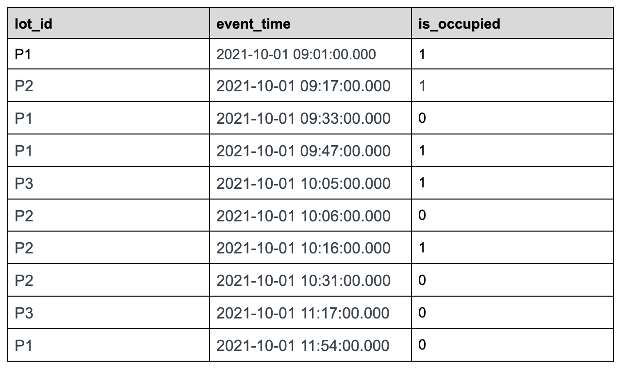
parking_data table

Use case: We want to find out the total number of parking lots that are occupied over a period of time, which would be a common use case for a company that manages parking spaces.

Let us take 30 minutes time bucket as an example:

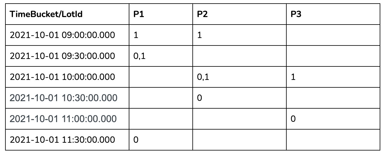
In the 30 mins aggregation results table above, we can see a lot of missing data as many lots didn’t have anything recorded in those 30-minute windows. To calculate the number of occupied parking lots per time bucket, we need to gap-fill the missing data for each of these 30-minute windows.

Interpolating missing data

There are multiple ways to infer and fill the missing values. In the current version, we introduce the following methods, which are more common:

• FILL_PREVIOUS_VALUE can be used to fill time buckets missing values for entities with the last observed value. If no previous observed value can be found, the default value is used as an alternative.
• FILL_DEFAULT_VALUE can be used to fill time buckets missing values for entities with the default value depending on the data type.

More advanced gapfilling strategies such as using the next observed value, the value from the previous day or past week, or the value computed using a subquery shall be introduced in the future.

Gapfill Query with a Use Case:

Let us write a query to get the total number of occupied parking lots every 30 minutes over time on the parking lot dataset discussed above.

Query Syntax:

SELECT time_col, SUM(status) AS occupied_slots_count
    FROM (
        SELECT GAPFILL(time_col,'1:MILLISECONDS:SIMPLE_DATE_FORMAT:yyyy-MM-dd HH:mm:ss.SSS','2021-10-01 09:00:00.000',
                       '2021-10-01 12:00:00.000','30:MINUTES', FILL(status, 'FILL_PREVIOUS_VALUE'),
                        TIMESERIESON(lot_id)), lot_id, status
        FROM (
            SELECT DATETIMECONVERT(event_time,'1:MILLISECONDS:EPOCH',
                   '1:MILLISECONDS:SIMPLE_DATE_FORMAT:yyyy-MM-dd HH:mm:ss.SSS','30:MINUTES') AS time_col,
                   lot_id, lastWithTime(is_occupied, event_time, 'INT') AS status
            FROM parking_data
            WHERE event_time >= 1633078800000 AND  event_time <= 1633089600000
            GROUP BY 1, 2
            ORDER BY 1
            LIMIT 100)
        LIMIT 100)
    GROUP BY 1
    LIMIT 100

This query suggests three main steps:

1. The raw data will be aggregated;
2. The aggregated data will be gapfilled;
3. The gapfilled data will be aggregated.

We make one assumption that the raw data is sorted by timestamp. The Gapfill and Post-Gapfill Aggregation will not sort the data.

Query components:

The following concepts were added to interpolate and handle time-series data.

• LastWithTime(dataColumn, timeColumn, ‘dataType’) – To get the last value of dataColumn where the timeColumn is used to define the time of dataColumn. This is useful to pick the latest value when there are multiple values found within a time bucket. Please see https://docs.pinot.apache.org/users/user-guide-query/supported-aggregations for more details.
• Fill(colum, FILL_TYPE) – To fill the missing data of the column with the FILL_TYPE.
• TimeSeriesOn – To specify the columns to uniquely identify entities whose data will be interpolated.
• Gapfill – Specify the time range, the time bucket size, how to fill the missing data, and entity definition.

Query Workflow

The innermost sql will convert the raw event table to the following table.

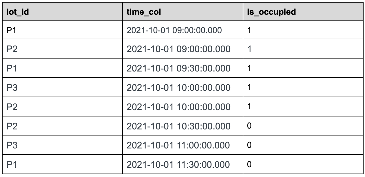
The second most nested sql will gap fill the returned data as below:

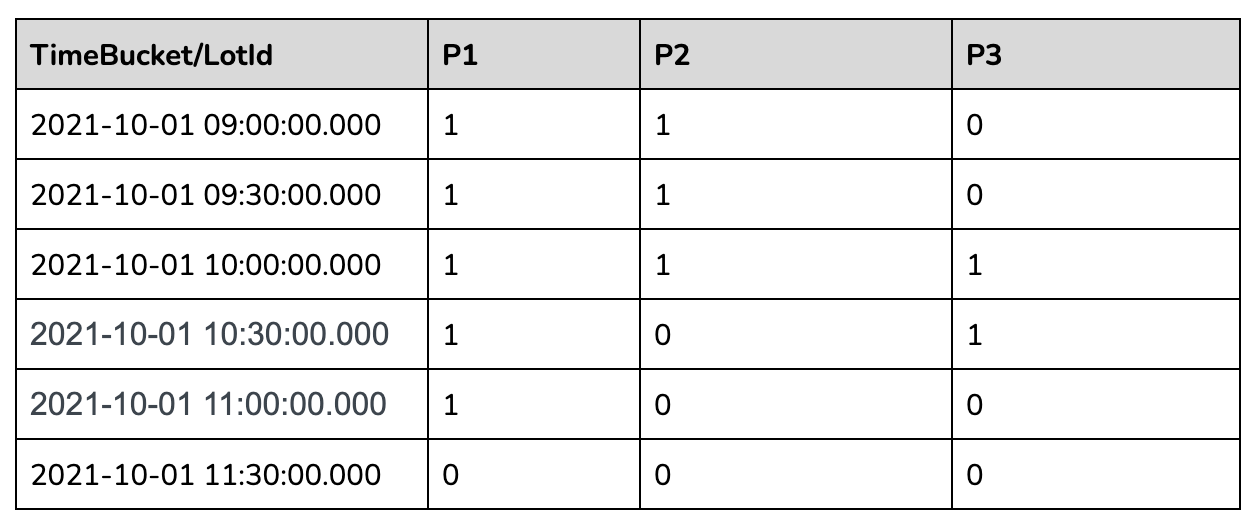
The outermost query will aggregate the gapfilled data as follows:

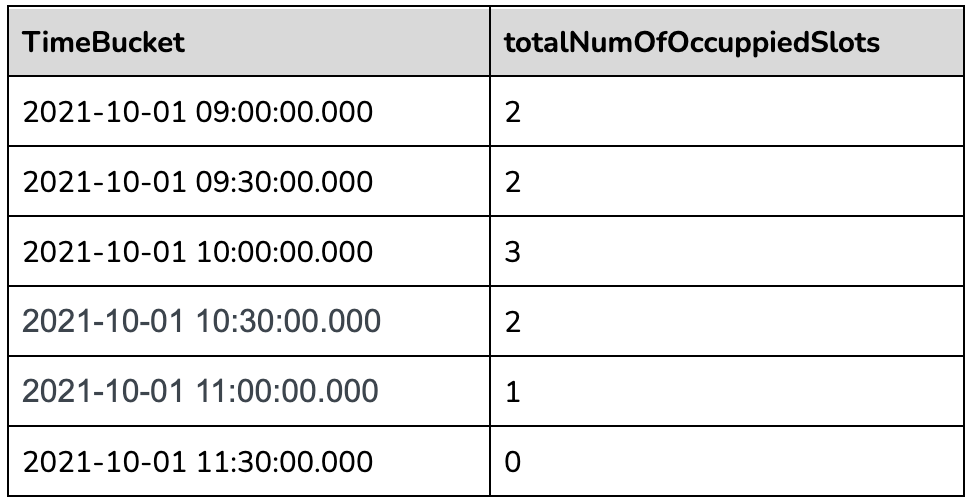
Other Supported Query Scenarios:

The above example demonstrates the support to aggregate before and post gapfilling. Pre and/or post aggregations can be skipped if they are not needed. The gapfilling query syntax is flexible to support the following use cases:

• Select/Gapfill – Gapfill the missing data for the time bucket. Just the raw events are fetched, gapfilled, and returned. No aggregation is needed.
• Aggregate/Gapfill – If there are multiple entries within the time bucket we can pick a representative value by applying an aggregate function. Then the missing data for the time buckets will be gap filled.
• Gapfill/Aggregate – Gapfill the data and perform some form of aggregation on the interpolated data.

For detailed query syntax and how it works, please refer to the documentation here: https://docs.pinot.apache.org/users/user-guide-query/gap-fill-functions.

How does it work?

Let us use the sample query given above as an example to understand what’s going on behind the scenes and how Pinot executes the gapfill queries.

Request Flow

Here is the list of steps in executing the query at a high level:

1. Pinot Broker receives the gapfill query. It will strip off the gapfill part and send out the stripped SQL query to the pinot server.
2. The pinot server will process the query as a normal query and return the result back to the pinot broker.
3. The pinot broker will run the DataTableReducer to merge the results from pinot servers. The result will be sent to GapfillProcessor.
4. The GapfillProcessor will gapfill the received result and apply the filter against the gap-filled result.
5. Post-Gapfill aggregation and filtering will be applied to the result from the last step.

There are two gapfill-specific steps:

1. When Pinot Broker Server receives the gapfill SQL query, it will strip out gapfill related information and send out the stripped SQL query to the pinot server
2. GapfillProcessor will process the result from BrokerReducerService. The gapfill logic will be applied to the reduced result.

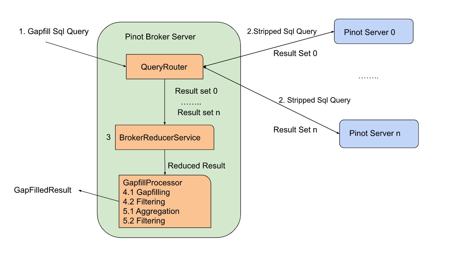
Here is the stripped version of the sql query sent to servers for the query shared above:

SELECT DATETIMECONVERT(event_time,'1:MILLISECONDS:EPOCH',
                   '1:MILLISECONDS:SIMPLE_DATE_FORMAT:yyyy-MM-dd HH:mm:ss.SSS','30:MINUTES') AS time_col,
                   lot_id, lastWithTime(is_occupied, event_time, 'INT') AS status
            FROM parking_data
            WHERE event_time >= 1633078800000 AND  event_time <= 1633089600000
            GROUP BY 1, 2
            ORDER BY 1
            LIMIT 100

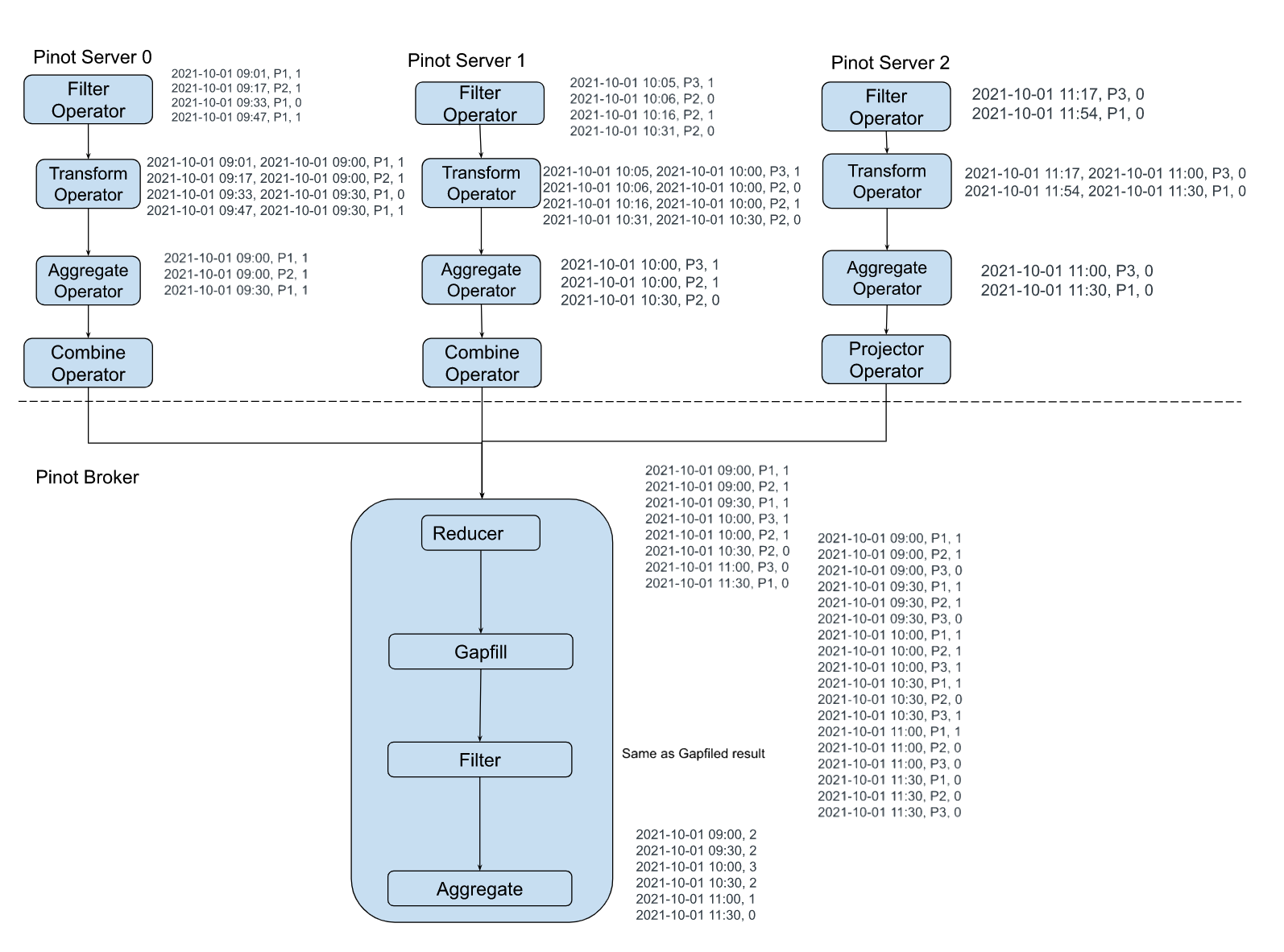
Execution Plan

The sample execution plan for this query is as shown in the figure below:

Time and Space complexity:

Let us say there are M entities, R rows returned from servers, and N time buckets. The data is gapfilled time bucket by time bucket to limit the broker memory usage to O(M + N + R). When the data is gapfilled for a time bucket, it will be aggregated and stored in the final result (which has N slots). The previous values for each of the M entities are maintained in memory and carried forward as the gapfilling is performed in sequence. The time complexity is O(M * N) where M is the number of entities and N is the number of time buckets.

Challenges

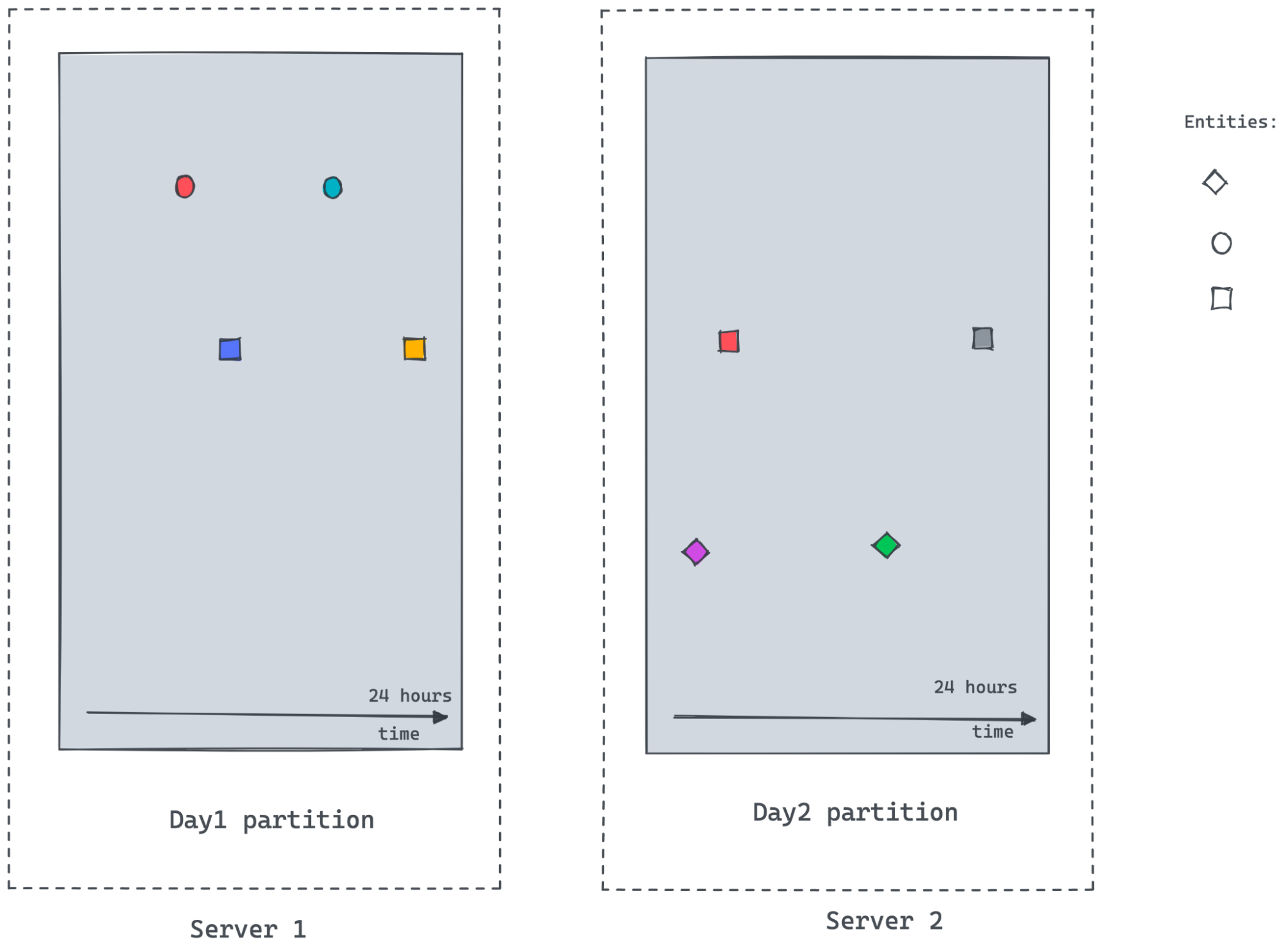
As the time-series datasets are enormous and partitioned, it’s hard to get answers to the following questions:

• How many different entities exist within the query time frame. In the temporal partition scheme demonstrated above, a server/partition may not know the answer.
• What’s the previously observed value for entities especially for the first data points in a time bucket where previous time buckets don’t exist in the same server.

For the scenario shown in the figure above, server2 may not know about the circle entity, as there are no events for the circle in Server2. It would also not know the last observed value for the square entity frame beginning of the time bucket till the first observed value timestamp within the partition.

The Future Work

When doing the gapfill for one or a few entities, there might not be too much data. But when we deal with a large dataset that has multiple entities queried over a long date range without any filtering, this gets tricky. Since gapfill happens at the pinot broker, it will become very slow and the broker will become a bottleneck. The raw data transferred from servers to brokers would be enormous. Data explodes when interpolated. Parallelism is limited as the single broker instance is handling the query.

The next step of the gapfill project is to remove the pinot broker as a bottleneck. The gapfill logic will be pushed down to the servers and be running where the data live. This will reduce the data transmission and increase the parallelism and performance of gapfill.