Visualizing Baseball Statistics with Apache Pinot and Redash

Analytics databases and data visualization are like hand in glove, adding tremendous value when used together. SQL queries return numbers, whereas visualizations make those numbers easy to digest at first glance, confirming the proverbial picture speaks a thousand words.

Apache Pinot, a real-time OLAP database, works with numerous BI tools to produce beautiful visualizations, including Apache Superset and Tableau. This article explores how Pinot can be integrated with Redash, another popular open-source tool for data visualization and BI.

What is Redash?

Redash is a data visualization tool built and maintained by an open-source community of 350+ contributors. Redash allows you to connect to different data sources, run queries, and build dashboards using charts of various formats: chart, cohort, pivot table, boxplot, map, counter, sankey, sunburst, and word clouds.

Redash natively integrates with many relational and NoSQL databases out there. Apart from that, Redash allows you to use a Python script as a data source, enabling you to populate the visualizations by running the script.

At the time of writing this, Apache Pinot doesn’t have a direct integration with Redash. Therefore, we will use Python script to write our queries and populate a dashboard.

Finding the hard hitters: the baseball stats dataset

Apache Pinot has a quick start example with a built-in schema, table, and sample records of baseball statistics. This data set has been derived from Sam Lahman’s famous baseball database. It contains complete batting and pitching statistics from 1871 to 2013, fielding statistics, standings, team stats, organizational records, post-season data, etc.

To keep things simple, let’s spin up an Apache Pinot Docker container in quick start mode to run our queries against the baseballStats table directly.

We will write queries to produce the following metrics:

1. Top ten players with all-time high run scores (rendered with a bar chart)
2. Top teams with all-time high run scores (rendered with a pie chart)
3. Total strikeouts by the year (rendered with a line chart)

Once we figure out the queries, we can write Python code in Redash to generate the required charts.

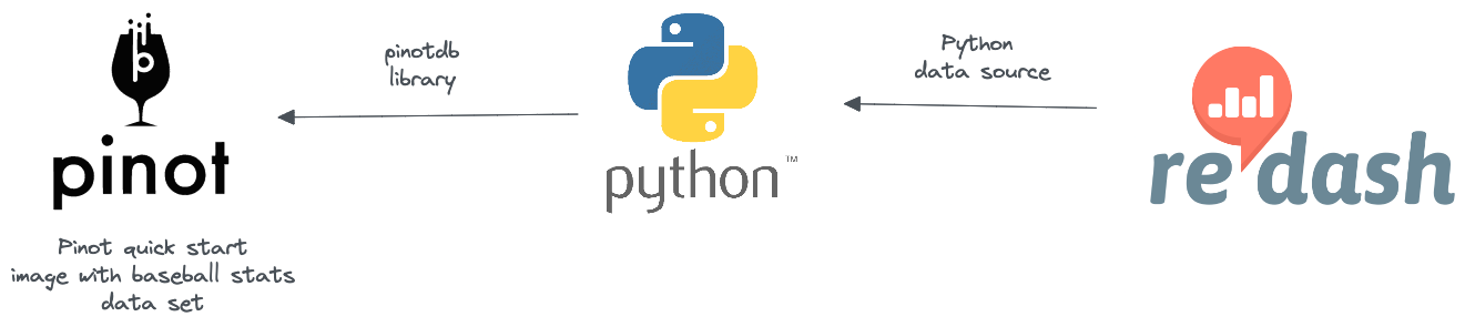
Figure 01 – Integration architecture

Step 1: Install Redash on your local machine

Redash comes with prebuilt machine images for cloud platforms, including AWS, Google Compute Engine, and DigitalOcean. It offers Docker Compose scripts as well.

Prerequisites

Here, we will install Redash locally using Docker Compose. Ensure your local machine meets the following requirements:

• Sufficient memory (more than 4GB)
• Docker Desktop installation.
• Install Node.js (14.16.1 or newer, can be installed with Homebrew on OS/X)
• Install Yarn (1.22.10 or newer): npm install –global yarn@1.22.10

Setup

First, you will need to clone the Redash Git repository:

git clone https://github.com/getredash/redash.git cd redash/

Redash requires several environment variables for operation. Create a .env file at the root and add the following content.

REDASH_COOKIE_SECRET=123456789 REDASH_ADDITIONAL_QUERY_RUNNERS=redash.query_runner.python

Note that the variable REDASH_COOKIE_SECRET must be set before you start Redash. The value of it can be anything. But there are some recommendations to follow.

We are going to query Pinot using Python scripts. Hence, the REDASH_ADDITIONAL_QUERY_RUNNERS is set to redash.query_runner.python.

Start the Docker services

Once you have the above set up, start the Docker container by running:

docker-compose up -d

That will build the Docker images, fetch some prebuilt images, and then start the services (Redash web server, worker, PostgreSQL, and Redis). You can refer to the docker-compose.yml file to see the complete configuration.

If you hit an errno 137 or errno 134, particularly at RUN yarn build , give your Docker VM more memory (At least 4GB).

Install Node packages

yarn --frozen-lockfile

If this command fails, a possible reason could be that you are running a newer version of Node. You can fix that by changing the Node version in the package.json file to match your Node version.

"engines": {  "node": "^16", 
 "yarn": "^1.22.10" 
 },

Create Redash database

Populate the Redash database by running the following command:

docker-compose run --rm server create_db

Build frontend assets

We still need to build the frontend assets at least once, as some of them are used for static pages (Redash login page and such):

yarn build

Once all Docker services are running, Redash is available at http://localhost:5000/ and should display the setup page as follows.

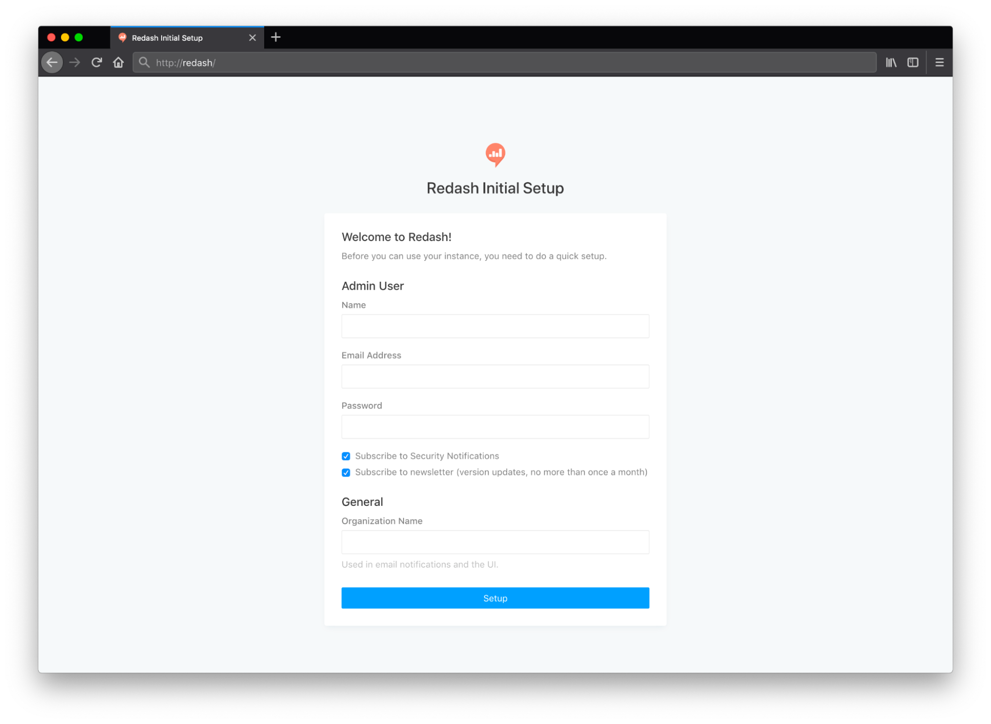
Figure 02 – Redash set up screen

Provide the admin username, email address, password, and organization name to proceed with this screen.

If you follow everything correctly, you should see a screen similar to this.

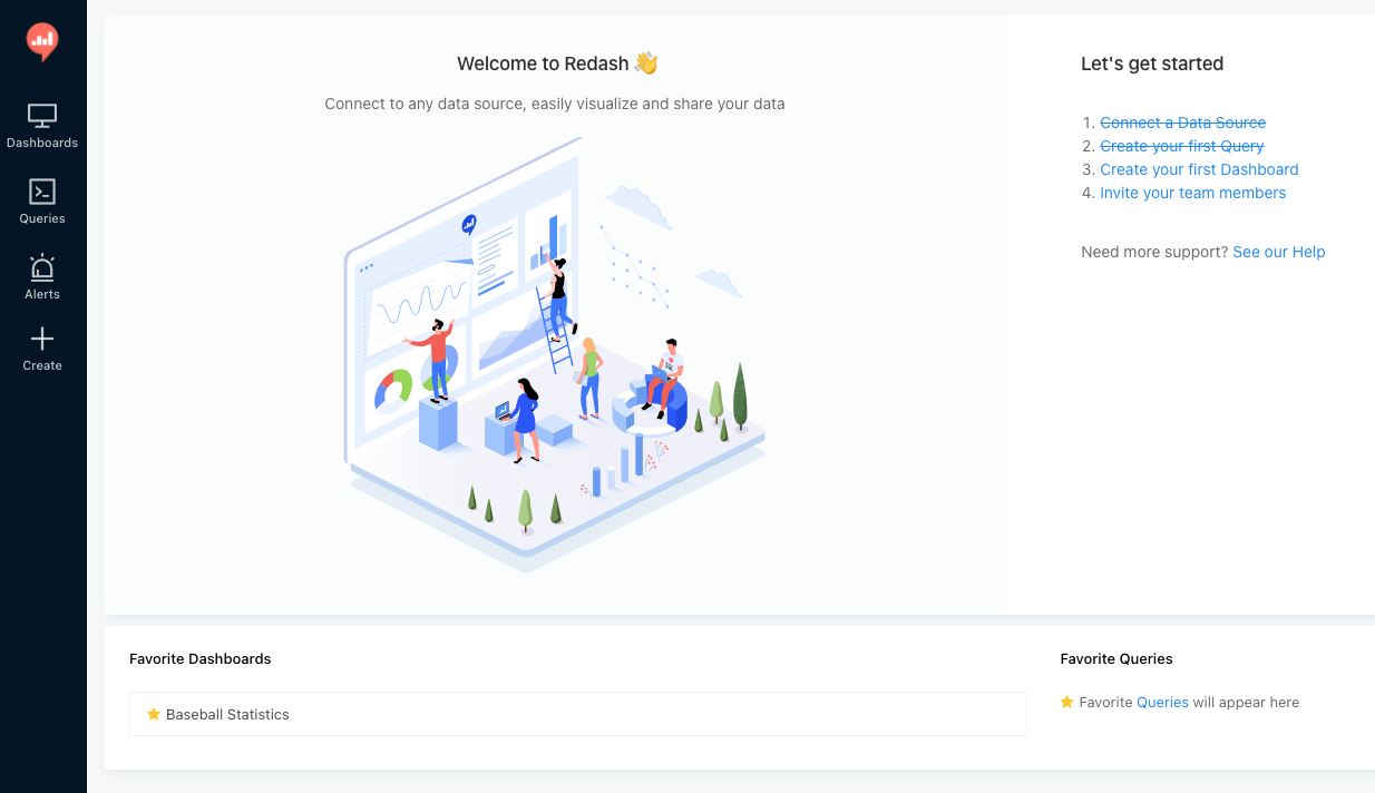
Figure 03 – Redash welcome screen

If you run into any issues during the installation, you can refer to this guide.

Step 2: Connect Pinot with Redash

Now that you have a running Redash instance. The next step is to configure Redash to query Pinot.

Add pinotdb dependency

Apache Pinot provides pinotdb , a Python client library to query Pinot from Python applications. We will install pinotdb inside the Redash worker instance so that it will be able to make network calls to Pinot from there.

Navigate to the root directory where you’ve cloned Redash. Execute the following command to get the name of the Redash worker container.

docker-compose ps

Assuming the worker’s name is redash_worker_1 , run the below commands to install pinotdb.

docker exec -it redash_worker_1 /bin/sh pip install pinotdb

Restart the Docker stack after installation.

Add a Python data source for Pinot

Go to Redash, select Settings > Data Sources , and select New Data Source . Then select Python from the dropdown list.

The Python query runner lets you run arbitrary Python 3 scripts and visualize the contents of a result variable declared in the script. The data source screen asks for three inputs.

• Modules to import prior to running the script let you define which modules installed by pip on the host server may be imported in Redash queries.
• AdditionalModulesPaths is a comma-separated list of absolute paths on the Redash server to Python modules that should be available when querying from Redash. This is useful for private modules that are not available from pip.
• AdditionalBuiltins Redash automatically allows twenty-five of Python’s built-in functions that are considered safe. You can specify others here.

Add pinotdb into the first text box as follows. Leave the others blank.

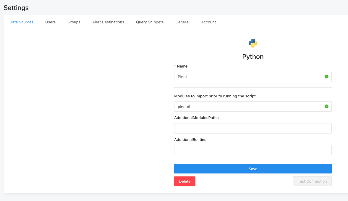
Figure 04 – Create the Python data source

Click on the Save button.

Step 3: Create visualizations

Now that we have a running Redash instance that can query Pinot. Let’s try to generate a few charts and add them to a dashboard.

Start Apache Pinot

Run the following command in a new terminal to spin up an Apache Pinot Docker container in the quick start mode. That container will have the baseball stats dataset built in.

docker run   --name pinot-quickstart  
 -p 2123:2123  
 -p 9000:9000  
 -p 8000:8000  
 apachepinot/pinot:0.9.3 QuickStart -type batch

Top 10 players by total runs

Go to Queries > New Query in Redash. Select the Python data source you created earlier.

Add the following Python code to the query editor.

from pinotdb import connect  
conn = connect(host='host.docker.internal', port=8000, path='/query/sql', scheme='http') 
curs = conn.cursor() 
curs.execute(""" 
 select 
playerName, sum(runs) as total_runs 
from baseballStats 
group by playerName 
order by total_runs desc 
limit 10 
""") 
 
result = {} 
result['columns'] = [ 
 { 
 "name": "player_name", 
 "type": "string", 
 "friendly_name": "playerName" 
 }, 
 { 
 "name": "total_runs", 
 "type": "integer", 
 "friendly_name": "total_runs" 
 } 
 ] 
 
rows = [] 
 
for row in curs: 
 record = {} 
 record['player_name'] = row[0] 
 record['total_runs'] = row[1] 
 
 
 rows.append(record) 
 
result["rows"] = rows

The above code connects to Pinot and queries the baseballStats table to fetch the top ten players with the highest scores. The result is then transformed into a dictionary format supported by Redash.

Click Execute to see whether the query returns any results. Click on the Add Visualization tab to add a Bar Chart as follows.

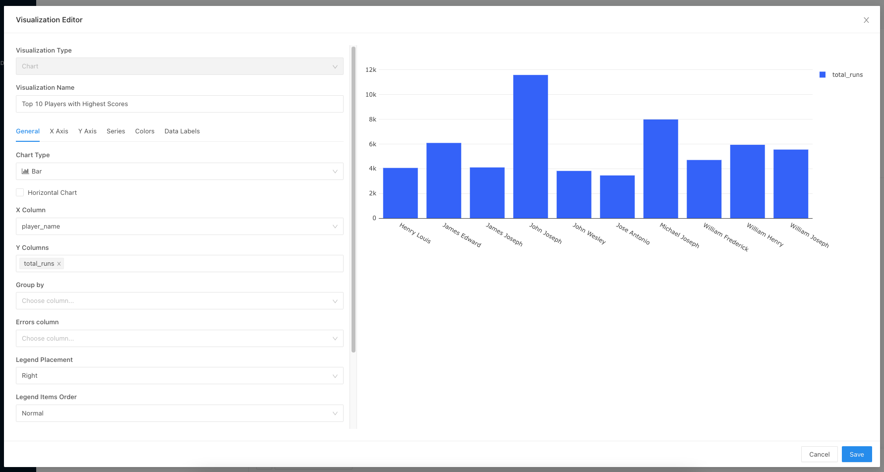
Figure 05 – Bar chart configuration

Click on the Save button to save the query with a meaningful name.

Top 10 teams by total runs

Similar to the above, add the following Python code to see the breakdown of teams who have scored the highest runs.

from pinotdb import connect  
conn = connect(host='host.docker.internal', port=8000, path='/query/sql', scheme='http') 
curs = conn.cursor() 
curs.execute(""" 
 select 
teamID, sum(runs) as total_runs 
from baseballStats 
group by teamID 
order by total_runs desc 
limit 10 
""") 
 
result = {} 
result['columns'] = [ 
 { 
 "name": "teamID", 
 "type": "string", 
 "friendly_name": "Team" 
 }, 
 { 
 "name": "total_runs", 
 "type": "integer", 
 "friendly_name": "Total Runs" 
 } 
 ] 
 
rows = [] 
 
for row in curs: 
 record = {} 
 record['teamID'] = row[0] 
 record['total_runs'] = row[1] 
 
 
 rows.append(record) 
 
result["rows"] = rows

You can add a pie chart as the visualization.

Total strikeouts by year

The following Python code returns the total strikeouts over time.

from pinotdb import connect  
conn = connect(host='host.docker.internal', port=8000, path='/query/sql', scheme='http') 
curs = conn.cursor() 
curs.execute(""" 
 select 
yearID, sum(strikeouts) as total_so 
from baseballStats 
group by yearID 
order by yearID asc 
limit 1000 
""") 
 
result = {} 
result['columns'] = [ 
 { 
 "name": "yearID", 
 "type": "integer", 
 "friendly_name": "Year" 
 }, 
 { 
 "name": "total_so", 
 "type": "integer", 
 "friendly_name": "Total Strikeouts" 
 } 
 ] 
 
rows = [] 
 
for row in curs: 
 record = {} 
 record['yearID'] = row[0] 
 record['total_so'] = row[1] 
 
 
 rows.append(record) 
 
result["rows"] = rows

You can create a line chart from the result as it shows the variation over time.

Create a dashboard

Finally, we can create a dashboard by piecing together the widgets generated by the three queries above.

Go to Dashboards > New Dashboards and add widgets accordingly. The final outcome should look like this:

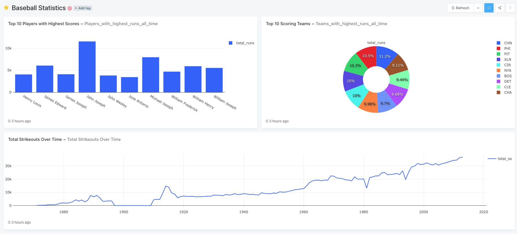
Figure 06 – Baseball stats dashboard

Summary

Although there’s no direct integration, for the time being, you can still use Apache Pinot with Redash via a Python data source. You will have to write queries in Python, which invokes Pinot broker through the pinotdb Python client library.

You can also include libraries like Pandas to perform more advanced data manipulation on Pinot’s data and visualize the output with Redash.

Apache Pinot Technology